Loudspeaker Measurements Standard: Our Procedure for Objectively Analyzing Speaker Performance

The presentation of loudspeaker measurements varies wildly from manufacturer to manufacturer.  This means that, without independent analysis, consumers are left comparing specifications that were obtained using completely different methods that yield different looking results.  In an effort to alleviate this confusion, it is our goal to provide readers with consistent measurement information for each loudspeaker reviewed allowing direct comparison from review to review.  As a part of this commitment, this article provides the nuts and bolts of the techniques used to measure loudspeakers. 

Before digging in, it is important to understand that the basic set of measurements described in this article is the minimum set of measurements obtained from each speaker reviewed going forward.  Since there are a ton of applications and form factors for speakers, it is sometimes necessary to provide additional measurements in the intended acoustic environment to provide a true picture of performance.  In all cases, loudspeakers will be measured using the process outlined here.  When supplemental measurements are taken, the review will clearly explain any deficiencies in the standard measurements due to the intended use.  As an example, if a loudspeaker is designed to sit on a desk, then its frequency response may incorporate the effects of the desk reflections and also the nearby wall behind it. If it is measured in free space without the reflections of the desk and rear wall, then it’s likely to exhibit a bass-shy response.  In this case, the standard measurement technique of measuring without the effect of the reflections may not provide an accurate picture of how the loudspeaker will perform for its intended use.  For this situation, additional measurements will supplement the standard measurements described here.

Audioholics Loudspeaker Measurement & Reviewing Process

The Audioholics Loudspeaker Measurement Standard will focus on the following measurement metrics:

• On-Axis Frequency Response
• Sensitivity
• Listening Window Response
• Polar Response
  
• Impedance & Electrical Phase
• Distortion Analysis

Our loudspeaker measurement standard provides the necessary foundation to getting as complete a picture as possible about how a loudspeaker objectively performs, not just at low listening levels but at high sustained output levels as well.

Loudspeaker Measurements Standard: On-Axis Frequency Response

On-axis frequency response is the starting place for measuring loudspeakers because it describes the initial sound that reaches a listener’s ear from a loudspeaker.  Although this response is the most revealing factor in determining how a loudspeaker sounds, it is only part of the complex auditory scene perceived by the listener.  Another part of the auditory scene is constructed from the interaction of a loudspeaker with the room that it is playing in.  Loudspeakers radiate sound into a room in various three-dimensional patterns that typically vary drastically as a function of frequency.  This causes a set of interactions only reproducible by, among other things, the combination of loudspeaker location, a specific listening environment and a precisely positioned listener.  The unique ear of the listener receives a barrage of acoustic information that is then converted into signals transmitted to the brain. The brain is a sophisticated signal processing system that more or less decides how the listener perceives the signals received.  Understanding how the brain processes sound is a topic of ongoing research and holds keys to advances in acoustics.

The frequency response of a loudspeaker can be obtained by first measuring the impulse response.  The impulse response, in theory, represents the output of the loudspeaker when presented with a pulse signal that lasts for an infinitely short amount of time.  Since there are some obvious issues with generating such a signal, it can be approximated using a maximum length sequence (MLS) consisting of pseudo-random pulses.  Circular cross-correlation of the MLS input with the loudspeaker output generates a good approximation of the system’s impulse response.  Assuming the loudspeaker is a linear time invariant (LTI) system, the time domain impulse response characterizes the loudspeaker frequency response through the properties of the Fourier transform.  Since this is all done using digital signals, the computationally efficient Fast Fourier Transform (FFT) algorithm is applied to obtain the Discrete Fourier Transform (DFT) of the impulse response.  For the interested reader, check out MIT’s cool tie wearing Alan Oppenheim’s course on discrete-time signal processing (MIT Open Course Ware - Discrete-time Signal Processing).

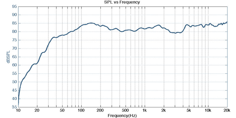
On-Axis Frequency Response Sample

The on-axis frequency response measurements are conducted with a 2.83VRMS excitation signal at a distance determined by proper summing of all drivers in the system.  This distance is determined by successively conducting the windowed measurement described below starting at 3 times the largest dimension of the source and decreasing the measurement distance in steps until one step before response deviations are apparent.  The SPL response for all measurements will be scaled to 1 meter mathematically.

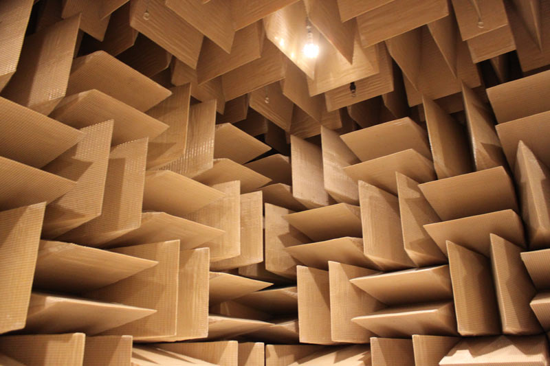
Anechoic Chamber - courtesy of Microsoft

Accurately measuring a loudspeaker’s impulse response is not a trivial task.  The difficulty lies in the fact that the measurements must be taken in a real space, and that space has some level of impact on the measurement.  One of the most useful places to conduct loudspeaker measurements is an anechoic chamber.  Anechoic chambers are large rooms with very thick sound absorption material on all surfaces and offer a good estimation of free-space measurements down to a cutoff frequency specific to the chamber.  Anechoic chambers can be calibrated to measure loudspeakers to frequencies below the cutoff frequency allowing full acoustic spectrum measurements. Unfortunately, they are very expensive to build.  Mere mortals are left measuring loudspeakers using quasi-anechoic techniques that are intended to approximate anechoic measurement techniques.

For measurements made in room, a signal processing technique called windowing is applied to only use the part of a measured impulse response that contains data before the first reflection of the sound from the nearest surface (usually the ceiling or ground). Calculating the length of the reflection free path and dividing by the speed of sound determines the reflection time. 

The reflection free path length is determined by the following equation:

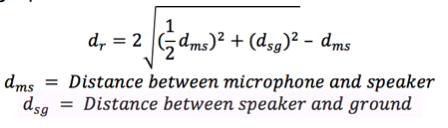
As an example, a speaker 1.14 meters off of the ground with a microphone distance of 1 meter yields a reflection free path length of approximately 1.49 meters.  The amount of time before the first reflection arrives is simply calculated by dividing the reflection free path length by the speed of sound.  This means that, in this example, we can use 4.3ms worth of the impulse response or frequencies as low as 230Hz considering the speed of sound is 344 m/s.  A window with a length equal to the gate time is applied to the impulse response. This gated response means that the measurement taken at 1 meter is only valid from 230Hz on up to 20kHz+.  Analogous to Heisenberg’s uncertainty principle, more accuracy in the window time yields less accuracy in the frequency response.  This means that, in the case of a 4.3ms window time, the frequency resolution is 230Hz yielding a small number of data points for low frequencies.  Software interpolates the missing data points but the results can potentially miss important variance in the low frequency data.

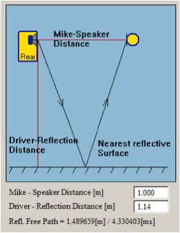
Mic Distance Diagram

There are several techniques used to obtain the low frequency data.  The first technique discussed is ground plane measurement.  This measurement technique involves positioning the loudspeaker such that the primary acoustic axis of the loudspeaker is facing the microphone placed on the ground in a large open space (typically outdoors).  For a single bass driver, the loudspeaker can simply be tilted vertically to align with the measurement microphone on the ground.  In the case of a multiple bass driver loudspeaker, the line of drivers should be parallel to the ground plane with the cones tilted directly at the measurement microphone with the highest frequency driver being measured directly on-axis with the microphone. 

The degree of tilt is equated as follows:

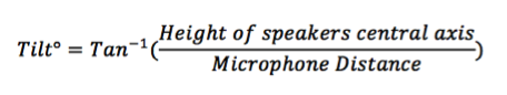
The height of the speaker’s central axis is typically the height of the center of the cone from the ground.  The microphone distance is the distance along the ground from the microphone to the acoustic center of the baffle.

Since the measurement microphone is approximately coincident with the ground, the measurement uniformly includes the reflected signal from the ground called the virtual image. This measurement technique typically introduces increasing error with increasing frequency.  Ground plane measurements may be conducted to obtain low frequency data to confirm the following near-field technique or when other techniques are impractical.

The second method, which can be used to obtain low frequency data for most loudspeakers, is the near-field measurement technique.  This technique involves measuring each low frequency element with the tip of the microphone very close to the driver.  This includes measuring bass drivers, passive radiators, and ports.

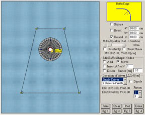
Baffle Step Modeling

For near-field measurements, the system baffle is modeled and baffle step diffraction simulations are conducted to approximate the effects of baffle step diffraction.  The wavelength of sound is a function of frequency with higher frequencies having shorter wavelengths.  This means that high frequencies reflect off of the baffle while low frequencies have a tendency to radiate spherically well beyond the width of the baffle.  As the wavelength increases (frequency decreases) and reaches the baffle width, the edge diffraction effects of the loudspeaker cabinet become an important consideration.  If the transition from hemispherical (2*pi) to spherical (4*pi) radiation is significant below the window frequency, the modeled baffle step diffraction will be combined with the near-field response data.  The modeled baffle step diffraction accounts for various driver alignments, baffle shapes and edge profiles.

 

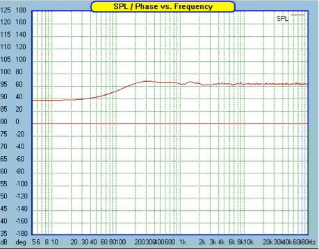
Baffle Step Diffraction Response

For near-field measurements, the same microphone gain settings are used for each measurement.  If a driver or port is located on the rear or side of the loudspeaker, the SPL is adjusted for the difference in distance from the reference plane.  The level matched near-field measurements and baffle step diffraction model are combined creating a single amplitude response including combined phase and accounting for diaphragm radiating areas.  The combined near-field response is then spliced with the gated response at approximately the window frequency.  The splicing technique requires level matching the low frequency data with the high frequency data before splicing together at a frequency below the crossover point of the driver’s measured near-field.  The technique requires finding a spot above the window frequency where the response contours and slopes match.  It is best to use the highest frequency possible to minimize the potential error due to the frequency resolution limit of the windowed response measurement.

 

 

Loudspeaker Measurements Standard: Sensitivity

Loudspeaker sensitivity is a measure of sound pressure level at a given distance when a specific sinusoidal voltage is applied across the loudspeaker terminals. The sound pressure level at the given voltage, say 2.83V, has to be inspected across the entire audio band.  Looking at frequency response, it is easy to see that for a constant voltage input, sound output varies with frequency.  It is easy to impress with this number by taking the peak in the loudspeaker frequency response and stating it as the loudspeaker sensitivity.  Unfortunately, this does not help anyone understand how loud the speaker will sound to the average listener.  Making all things fair, it is better to find the average SPL from 300Hz to 3kHz representing the mid-band of a typical full range loudspeaker. 

Editorial Note about Sensitivity Frequency Range by Dr. Floyd Toole:

This frequency range was selected because it embraces most of the significant frequencies in human voices and much music.

This is the method accepted by the well-respected National Research Council of Canada, so we are sticking with it!  In the rare case where 300Hz to 3kHz is not in the mid-band of the speaker under test, additional information will be included in the review assessing the sensitivity based on the mid-band range of the speaker.

The sensitivity measurement is obtained from the on-axis frequency response measurement.  Prior to the measurement, the microphone is calibrated at 94dB and 114dB reference points established by an acoustical calibrator.  A 2.83VRMS MLS signal is applied to the loudspeaker and the measurement captures the SPL calibrated frequency response.  The output is exported to mathematical software capable of working with matrices for averaging the SPL.  Since SPL is a logarithmic scale, the average of the inverse logarithm of each value must be equated and converted back to decibels.

For more information on this topic, see:  Loudspeaker Sensitivity Specifications & Measurements Explained

Listening Window

Unfortunately, there is only one sweet spot and sometimes the listening chair does not position the listener at the same height as that sweet spot.  That is why listening window measurements are so important.  A listening window measurement Audioholics style is simply an average of loudspeaker measurements at the reference distance from 7 different locations. 

• On-axis
• +/- 15 Degrees Horizontal
• +/- 30 Degrees Horizontal
• +/- 15 Degrees Vertical

 

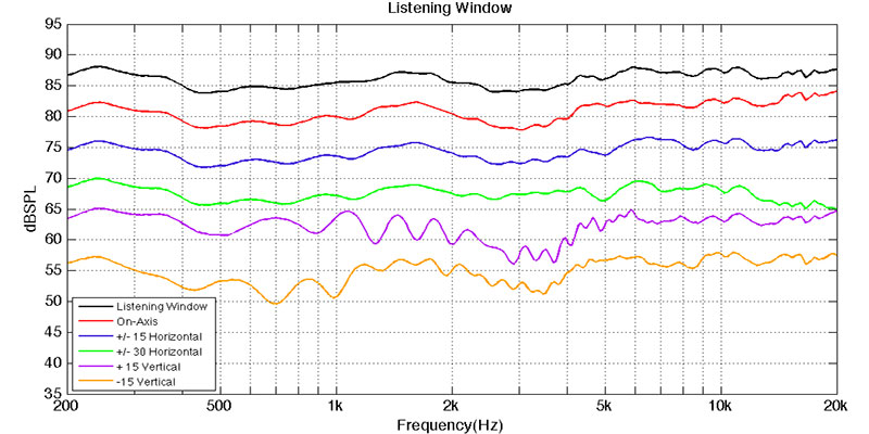
Listening Window Sample

This gives you an idea of the power response of the system.  If on-axis measurements look great but the listening window is not even close, then the sweet spot will be relatively narrow.  The published listening window graph shows the response at each angle independently so that you will have an idea of how the speaker will sound in typical listening positions.

The results for a listening window measurement are obtained using 2.83VRMS at the reference distance and moving the measurement microphone to the specified angle.  The low frequency response below the window frequency is typically relatively uniform so it is not included in the measurement.

Polar Response

Polar response measurements are obtained by measuring the loudspeaker from 0 to 180 degrees in 7.5 degree increments following the same methods used to obtain on-axis frequency response at the reference distance.  The vertical axis of rotation is the acoustic center of the baffle.  In cases where the loudspeaker does not have vertical symmetry, the measurement is taken from 0 to 360 degrees.  Polar response measurements from 0 to 90 and 90 to 180 degrees are contour plotted in software for a clear representation of polar response versus frequency for the forward plane and rear plane of the loudspeaker.  This information can be used to determine loudspeaker directivity, room interactions, off-axis listening and gives a general idea about the power response of the loudspeaker in the horizontal plane.

 

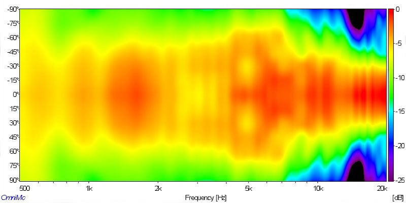
Polar Response Sample

Impedance and Electrical Phase

Impedance measurements are conducted using a very simple technique.  A resistor of a known (measured) value is placed in line with the positive speaker terminal.  Two voltage probes connected to a soundcard are connected to the amplifier side of the resistor.  A 1kHz test tone is sent to the loudspeaker and the difference in the sensed voltage is automatically calibrated out in the measurement software.  Next, one of the measurement probes is moved to the speaker side of the known resistor and an MLS sequence is generated.  The impulse response of the impedance and phase is captured and converted to the frequency domain using the same techniques discussed in the on-axis frequency response section.

 

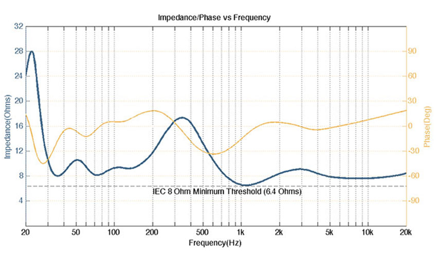
Impedance and Electrical Phase Sample

The impedance of a loudspeaker is important when trying to mate a loudspeaker with an amplifier.  An ideal audio amplifier should output a constant voltage regardless of the impedance of the speaker.  However, no amplifier can produce infinite current.  Using Ohm’s law, it is clear that as impedance decreases the current must go up in order to hold voltage constant.  Many amplifiers are not designed to handle impedances below 6 ohms due to the increased current draw.

The lowest impedance is measured at DC, which is also known as the DC resistance. The IEC 26-8 method of specifying nominal loudspeaker impedance is set such that minimum impedance must not fall below 80% of nominal, so for an 8 ohm speaker this would be 6.4 ohms minimum, and for 4 ohms would be 3.2 ohms.

The impedance phase is an important factor to look at as well, because it relates to how efficiently the amplifier can deliver power to the loudspeaker.  When the phase angle of the impedance is greater than 0 degrees, the loudspeaker is presenting a partially inductive impedance to the amplifier which typically does not pose much threat to amplifiers.  When the phase angle is less than 0 degrees, the loudspeaker is presenting a partially capacitive impedance to the amplifier.  A large capacitive load can cause instability in some amplifiers.

Distortion Testing

Harmonic distortion components are generated by exposing a loudspeaker to a stepped sinusoid excitation signal and measuring the system’s response. To reduce the effects of noise on harmonic distortion measurements, the software uses heterodyne filters to select the harmonic frequency being measured.  The total harmonic distortion measurement is displayed in percent representing the percentage amplitude of harmonic distortion present compared to the fundamental.

This measurement is conducted on axis with a stepped sinusoid excitation signal at 90dB measured from 2-meters.  The 2^nd through 5^th harmonics are graphed together with the total harmonic distortion (THD) showing the constituent parts of the total harmonic distortion.

Analysis of the THD results should be taken in the context of the loudspeaker under test. Note that the distortion percentage is a logarithmic scale. The components listed as D2-D5 represent the 2^nd through 5^th harmonic of the fundamental.  The graph shows the amount of each harmonic present at the given fundamental frequency.  So the contribution to distortion from the 2^nd harmonic of a 1kHz signal is visible by finding the line for D2 at 1kHz.  In this case, D2 represents two times the fundamental frequency, which is 2kHz.  Due to the limitations of the measurement/playback system and human hearing, harmonic frequencies above 24kHz will not be measured.  Since a harmonic is an integer multiple of the fundamental frequency, the harmonic distortion plot for each harmonic stops when the product of the harmonic order number and the fundamental frequency equals 24kHz.

 

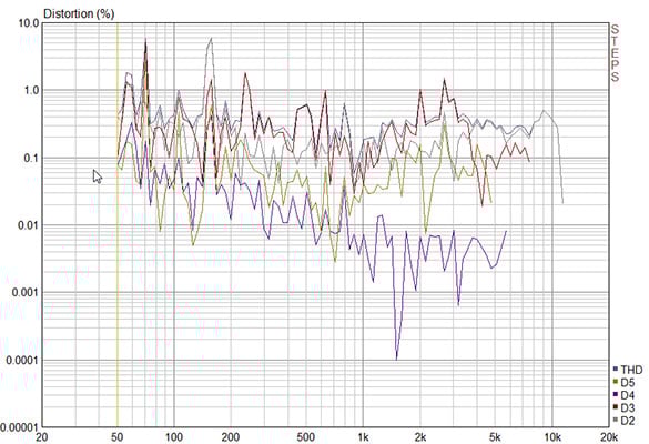
Harmonic Distortion % Sample

Harmonic distortion is a standard test applied to many systems handling signals.  However, the correlation between harmonic distortion numbers and the human perception of sound quality is very poor.  This is because harmonics are typically masked in the broadband music signal.  Additionally, harmonics do not sound as bad as frequencies that are not integer multiples of the fundamental.  Inter-modulation distortion is another type of distortion that is produced when a loudspeaker plays multiple frequencies simultaneously.  Inter-modulation distortion is particularly offensive because it creates distortion at frequencies that are sums and differences of a mixed signal.  The frequencies produced are not musically correlated with the fundamentals that produced them.  Audioholics is actively researching methods to measure and display inter-modulation distortion that are presentable and useful to readers.

Cumulative spectral decay is a very easy way to identify loudspeaker resonance issues.  If a cabinet or driver has an issue with resonance in the audible band, the cumulative spectral decay plot shows how the response of the loudspeaker decays from an impulse excitation signal versus frequency.  As was discussed in the On-Axis Frequency Response section, the discrete Fourier transform of a gated impulse response generates frequency response.  To see the decay, the window is simply moved forward a certain amount of time and the discrete Fourier transform is calculated using the fast Fourier transform successively until the reflection free window time is reached.  This measurement is obtained at 2.83VRMS at the reference distance discussed in the on-axis frequency response section.  The sample results show the low frequency data cutoff curling to higher frequencies, this is due to the moving window. 

Editorial Note Regarding CSD by Dr. Floyd Toole:

Because of the time gating, necessary to see into the time domain, frequency resolution is sacrificed – note the smoothness of the curves. This means that energy in a high-Q resonance is spread over a wider frequency range, resulting in an artificially low level.  Besides all of this decorous displaying of data, the fact is that, except at very low frequencies, humans do not hear the ringing, we hear the spectral bump (which, ironically in these displays cannot be accurately seen).  See Section 9.2.1 in my book [1]. See also Figure 13.23 p. 246 for examples of the “uncertainty” principle as applied to waterfall displays of data.  You have a choice of seeing high resolution in time or frequency domains, not both.  They are pretty, though.

In perceptual terms, the audibility of ringing is substantially reduced by a phenomenon known as “forward temporal masking” – the initial sound reduces the audibility of sounds that immediately follow it.

[1] F. Toole, Sound Reproduction: Loudspeakers and Rooms. Burlington, MA: Elsevier, 2008

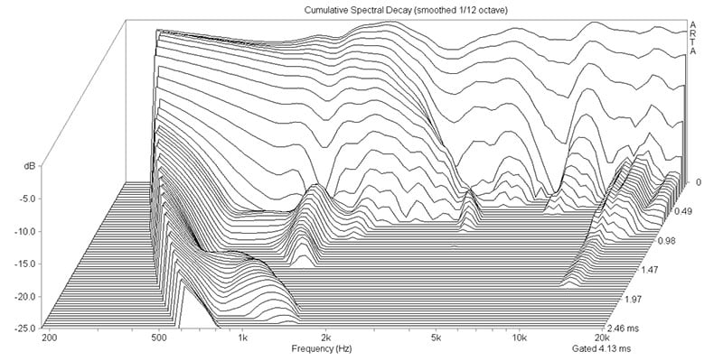
CSD Sample

The group delay of loudspeakers is also analyzed.  Group delay can be derived from the impulse response measurement and represents the time delay of amplitude envelopes of sinusoidal components through a loudspeaker.  While harmonic distortion is typically displayed in the frequency domain, group delay distortion is displayed in the time domain.  The group delay measurement defines the rate of change of the slope of the loudspeaker phase.  Group delay values between 1.6 to 2.0 ms [1] in the mid to high frequencies are detectable but their effect on the perception of sound quality is not well established.

 

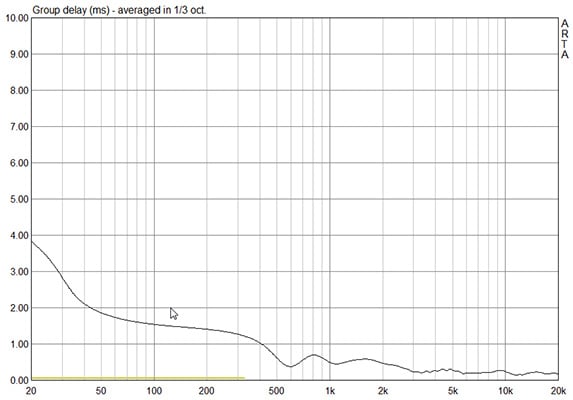
Group Delay Sample

 

Additional Tests

As part of the review process, each loudspeaker is disassembled.  The loudspeaker drivers, cabinet construction, and crossover components are inspected.  Each individual driver is measured independently in the cabinet to determine crossover frequencies, crossover slope and each driver’s contribution to the system response.  If anything interesting or out of the ordinary is determined, additional graphs will be generated.

Loudspeaker Measurements Standard: Equipment & Calibration

Obtaining useful loudspeaker measurements has never been easier than it is today.  Measurement results can be obtained using computer-based measurement software, a quality two-channel recording audio interface, a calibrated measurement microphone and a little patience.  We use the following equipment and software to conduct loudspeaker measurements:

• SoundEasy V18 by Bodzio Software 
• ARTA/STEPS by Ivo Mateljan 
• RME Fireface 800 Firewire Audio Interface
• ATI AT6012 Audio Amplifier
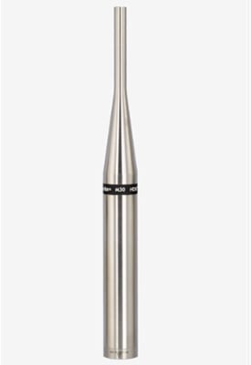
• Earthworks M30 Omnidirectional Measurement Microphone
• Sper Scientific 2 Point Acoustical Calibrator (850016)
• Dayton Audio OmniMic V2 Precision Measurement System
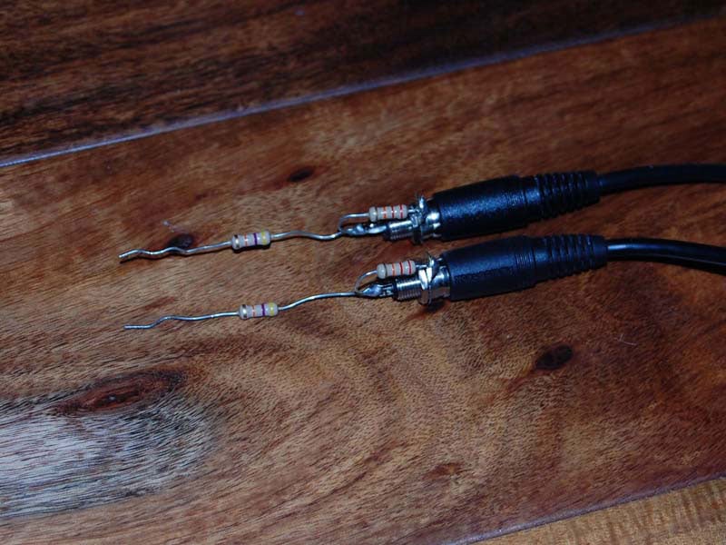
• Hand Built Impedance Measurement Probes
• Radio Shack Digital Multimeter with RS-232 output

SoundEasy is a very powerful loudspeaker modeling, design, and measurement package. This package includes components for obtaining frequency response, phase, impedance and distortion measurements, to name a few.  For those interested in loudspeaker design, this package has an excellent price-to-performance ratio and covers all of the bases imaginable, including finite element method, non-linear driver analysis, T/S parameter extraction, analog crossover design, digital crossover design, cabinet modeling and much more. The manual is actually a great resource for those interested in learning more.  Just keep in mind it is not for the faint of heart, the manual is 525 pages and covers some topics that are heavy in mathematics. 

ARTA software is a very easy to use impulse response measurement package that provides a cost effective method to obtain loudspeaker frequency response, cumulative spectral decay and other frequency domain information.  STEPS is bundled with ARTA and provides swept sine measurements for generating the distortion measurements used here.  While SoundEasy also provides this functionality, it is much more involved to obtain measurements and the output graphs are not as attractive for publishing purposes. 

The RME Fireface 800 is a high-quality 56-channel audio interface including analog preamplifiers,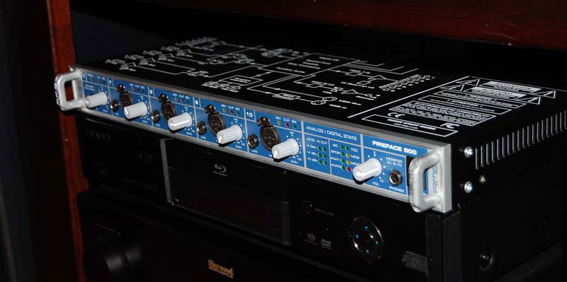 phantom microphone power, an excellent computer mixing interface and industry leading device drivers.  This equipment is used to reliably convert the analog measurement information from the impedance probes and measurement microphone into the format needed by the measurement software.  Additionally, it serves as the audio source for excitation signals required for measurement.

The ATI AT6012 is a 12-channel power amplifier used for measurements.  The amplifier is used because it is flexible, reliable and has excellent performance.  The AT6012 is capable of driving very low impedance speakers and provides very good voltage stability.  In cases where speakers must be bi-amplified or tri-amplified for testing, the AT6012 amplifier has sufficient current to drive all channels simultaneously at the voltage levels required for testing.

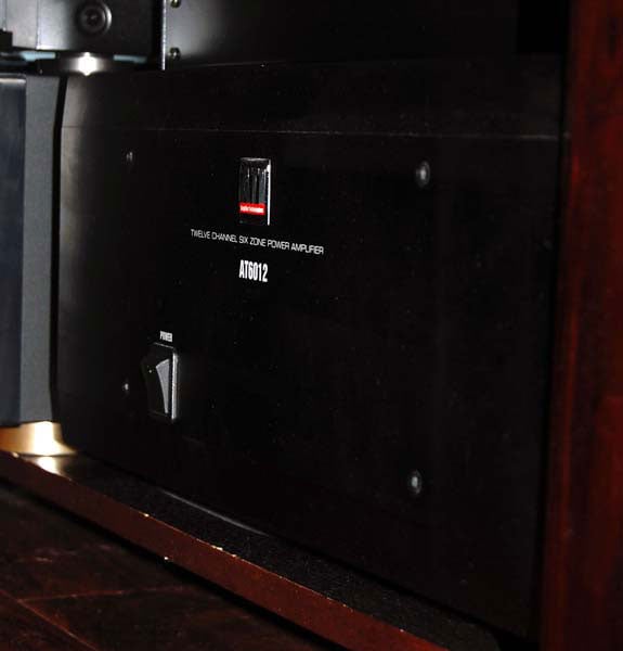
                                        ATI AT6012

The Earthworks M30 omnidirectional measurement microphone was selected for all acoustical measurements.  This decision was made based on the M30’s solid reputation and specifications such as ruler flat and extended frequency response.  Although the microphone is +1/-3dB from 5Hz to 30kHz without a calibration file, the included calibration file will be used for all loudspeaker measurements.  If you find yourself needing to measure a jet engine, the 142dB maximum input might come in handy.  If your measuring something like loudspeakers, the low self-noise and excellent distortion performance may be more useful.

Even though the Earthworks M30 is a calibrated measurement microphone, there is no way to determine absolute sound pressure levels without a point of reference.  This is because the RME Fireface does not have a reliable zero gain setting on the preamplifier.  Thus, the simplest solution to determining absolute SPL is use of an acoustical calibrator.  Leveraging the expertise of Herb Singleton at Cross Spectrum Labs, the Sper Scientific acoustical calibrator was selected. Cross Spectrum will independently validate the accuracy of the acoustical calibrator and the M30 calibration as needed.

 

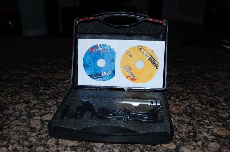
Dayton Audio OmniMic System (left pic) ; Earthworks M30 Microphone (right pic)

 

Dayton Audio OmniMic V2 Precision Measurement System is quite a mouthful.  This is a bread and butter no-nonsense package that provides just what most folks need for measurement without all of the cost of a software package, audio interface and a calibrated microphone.  It’s simply a calibrated USB measurement microphone with a software package and test tone disc that is exceedingly simple to use.  It gives access to frequency response measurements, SPL measurements, distortion analysis, room analysis, bass decay and the very nice polar response graphs used in our loudspeaker reviews.  This package is not for a professional loudspeaker designer, but is definitely useful for someone trying to tune a system or analyze speakers.

To perform impedance measurements on loudspeakers, a pair of probes is required.  The probes connect to the line input of the soundcard and measure the current through a known resistor by measuring the voltage drop across the resistor (if you’re confused, see Understanding Ohm's Law, Impedance and Electrical Phase 101 ).  The probes are very simple, consisting of ¼” mono phone connector to RCA jack.  The end of the RCA jack has a 47k ohm resistor from center to ground and a 22k ohm resistor in the signal path.  The probes provide a method to safely determine voltage differences using a standard sound card.

The Radio Shack Digital Multimeter (DMM) with RS-232 serial output is a necessary tool for obtaining measurement and calibration parameters.  The RS-232 output links to computer software that provides the DMM output directly on the measurement computer screen.  This is extremely convenient while trying to set and test voltage levels at different loudspeaker playback levels.  As needed, the multimeter readings are compared to a Tektronix TDS3000 series oscilloscope with an input signal of 2.83VRMS at 60Hz, 120Hz and 500Hz to validate accuracy.

 

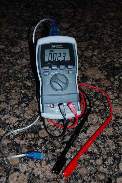
RadioShack Multimeter with RS-232

Calibration Routine

SoundEasy has a spectrum analyzer plug-in that has a built-in signal generator.  The signal generator can provide single/multi-tone sine signals, pink noise, white noise, square waves, tone bursts or custom sound files.  The first step in calibration is to determine the soundcard and SoundEasy volume level required to generate 2.83VRMS across the loudspeaker terminals.  Using the Radio Shack DMM display, each is adjusted until 2.83VRMS is displayed with no load attached with a 60Hz input signal.  The input signal is then increased to 120Hz and then to 500Hz to confirm the voltage output of the amplifier is stable versus frequency.  Next the loudspeaker is attached and the voltage stability is confirmed at 60Hz, 120Hz and 500Hz.  The values of the digital volume control in SoundEasy and the Fireface software are recorded.  This routine is then repeated for 8.944VRMS and 14.14VRMS across the loudspeaker terminals representing 10W and 25W into 8 purely resistive loads.

Since the RME Fireface and Earthworks M30 do not have a reference for absolute SPL measurements, the Sper Scientific acoustical calibrator is used to produce a reference 94dB and 114dB. The tip of the M30 measurement microphone is placed in the acoustical calibrator and exposed to a 94dB reference signal.  The spectrum analyzer plugin in SoundEasy is used to adjust the RME preamplifier gain until the reference level of 94dB is measured in SoundEasy.  The acoustical calibrator is changed to the 114dB setting and the input level is confirmed in SoundEasy.

Glossary of Terms

• Analog Crossover – Set of active or passive filters used to split an analog audio signal into frequency bands appropriate for each driver of a loudspeaker.
• Anechoic Chamber – A room in which reflections above a given cutoff frequency are attenuated to a level where they do not significantly affect the measurement of direct sound from a loudspeaker.  The cutoff frequency decreases as the thickness of the absorption material increases.
• Baffle Step Diffraction – Inherent change in output of a loudspeaker as the wavelength of sound increases beyond the width of the loudspeaker baffle .
• Bass Decay – Describes how long it takes bass frequencies to reduce in amplitude after being played into a room.  This is primarily determined by the Q of room resonance modes.
• Cumulative Spectral Decay – A series of frequency response slices cascaded to show how sound reduces in amplitude with respect to time.  Cumulative spectral decay graph resolution is inversely related in the time and frequency domains.
• Digital Crossover – Use of digital signal processing techniques to split a digital audio signal into frequency bands appropriate for each driver of a loudspeaker.  This technique allows more complex filter designs and better matching of transducer requirements than an analog crossover counterpart.  The split signals must be converted to analog and amplified before being transmitted to the loudspeaker.
• Distortion (Loudspeaker) – Broad term describing both linear and non-linear change in the transmitted content of an electrical or acoustic signal during transmission.
• Electrical Phase – A property of loudspeaker drivers in combination with a crossover that causes leading or lagging of current relative to voltage where high phase angles equate to less efficient delivery of power to a loudspeaker.
• Finite Element Method (Acoustics) – Process used to solve complex equations relating to modeling the acoustics of a room to determine modes and sound pressure levels at various locations.
• Frequency Response – A graph showing sound pressure level as a function of frequency
• Group Delay - The time delay of amplitude envelopes of sinusoidal components through a loudspeaker.
• Gating – A signal processing technique in which the duration of the impulse response used to calculate the amplitude response is limited in time.  This technique is widely used for acoustical measurements conducted in an environment that produces reflections to limit the impact of reflections in the measurement.  The trade-off is reduced frequency resolution causing loss of information at low frequencies.
• Impedance – Electric or acoustic property that quantifies a loudspeaker’s frequency dependent resistance to an alternating effect such as an alternating voltage input signal.
• Impulse Response – A time domain measurement of a system’s response to an impulse of very short duration.  In practice, the impulse is required to have a duration much smaller than the period of the highest frequency of interest.
• Maximum Length Sequence (MLS) – A pseudo random binary sequence that is spectrally flat and is an ideal excitation signal for impulse response measurement.
• Multimeter – A device that measures electrical properties of voltage, current and resistance using two probes.
• Pink Noise – Broadband excitation signal that contains an equal amount of noise power per octave (per percentage bandwidth).
• Polar Response – Frequency response of a loudspeaker measured at some number of frequencies, at many angles over a horizontal and/or vertical orbit.  The results may be plotted as a continuous polar graph of sound level versus angle for individual frequencies or bandwidths, or as a family of frequency responses plots at designated angles.
• Quasi-Anechoic – Techniques used to approximate measurements made in an anechoic chamber while in a reflective or reverberant field.
• Room Analysis – Consideration of a room’s acoustic properties in the design of a sound system.
• Signal Generator – System that provides an output signal matching a user's desired input requirements including wave shape, frequency and amplitude.
• Spectrum Analyzer – Tool used to analyze signals in their frequency domain components.
• Sound Pressure Level – A standardized measure, in decibels (dB) in which a sound level is stated with relation to an internationally agreed upon reference sound pressure level.
• Square Wave – A periodic signal that theoretically transitions from off to on and on to off instantly spending equal amounts of time off and on.
• T/S Parameters – Thiel/Small parameters are loudspeaker driver parameters that quantitatively identify a loudspeaker’s small-signal performance and provide a mathematical method to estimate a driver’s performance in an enclosure.
• Total Harmonic Distortion (THD) – Harmonic distortion is loudspeaker distortion having distortion products at integer multiples of the fundamental frequency.  Total harmonic distortion is a single number combining all harmonic distortion products.
• Voltage Sensitivity – Describes the sound pressure level (SPL) at a standardized distance of 1 meter for a standardized input of 2.83VRMS.  Voltage sensitivity is used over efficiency because good power amplifiers behave as constant voltage sources.
• Voltage Stability – Ability of an amplifier to maintain a constant voltage output regardless of the load impedance.
• White Noise - Broadband excitation signal that contains an equal amount of noise power per Hertz (per fixed bandwidth)
• Windowing - See gating.

Acknowledgements

We would like to personally thank the following people for their contributions and/or peer review of this article, all of whom are true experts in their respective fields. Their contributions enabled us to make the most comprehensive and accurate article possible on the very complex topic of loudspeakers cabinets dealt with herein.

• Steve Feinstein, Audio Industry Consultant
• Ed Mullen, Directory of Technology & Customer Relations of SV Sound
• Dennis Murphy, Loudspeaker Designer of Philharmonic Audio
  
• Shane Rich, Technical Director of RBH Sound
• Mark Sanfilipo, Audioholics.com Resident Speaker Expert and Writer
• Dr. Floyd Toole, Former VP of Acoustical Engineering of Harman; published author of "Sound Reproduction, The Acoustics and Psychoacoustics of Loudspeakers and Rooms", Focal Press, 2008.
• Product Development Engineer, Atlantic Technology