
Audioholics Subwoofer Measurement Standard Part I
When it comes time to size up a subwoofer's performance, the proof is in the measurement! Audioholics takes a hard look at the science of subwoofer measurements in a two-part series covering a broad spectrum of measurement methods, useful to both pro and enthusiast alike. Let the science begin!"
This article began life as an ongoing series of conversations, carried out over the past couple of years with Gene. He recognized Audioholics’ need to bring a degree of organization to its own in-house subwoofer measurement procedures. I was tasked with that challenge and present here Part I.
Part II, to be published later, will cover other topics such as linear & nonlinear distortion measurement, mechanical noise floor measurement, amplifier measurement and so forth. Part II will also include a collection of worked examples and conclude with a table summarizing all results.
Projects of this size are seldom a
solo effort and this was no exception. To that end, a huge debt gratitude
is owed to Charlie Hughes, Jeff Szymanski,
Siegfried Linkwitz, Don Keele, Neville Thiele and many others who contributed
their time and expertise in helping me knock this manuscript into shape. Thank
you, gentlemen! And of course, a big thanks to Gene as well for his almost
supernatural patience as he waited for me to bring this to completion. Thanks,
Gene!
Scope
The purpose of both documents is to present a set of measurement guidelines by which a comprehensive objective assessment of a subwoofer’s performance can be developed. Included within this document’s definition of a subwoofer are: single & multiple driver subwoofer systems; powered and passive systems; systems featuring vented or totally enclosed cabinets; along with less common items such as dipole subwoofers.
Though industry professionals can (and do) make use of the methods or approaches presented here, this document is intentionally structured and organized to make it particularly useful to the audio enthusiast. Given the particular type and/or characteristics of a sub you may be interested in measuring you may find it unnecessary to apply all the measurement procedures covered in Parts I & II. In any event, with the variety of software-based measurement tools currently available, it is now possible for the audio enthusiast to work up a collection of accurate measurements at very little expense. Certainly much less expensive than what it would have cost 20 or 30 years ago!
If you’ve spent any time at all contributing to the development of any sort of industrial standard, you’ll know the process tends to be evolutionary in nature. Similar in character to the more formal standards (AES, IEC, etc) from which parts of this work are drawn, nothing here is written in stone. As new research and/or measurement technologies/techniques appear on the horizon they will be included, whenever/wherever appropriate and/or applicable. This is a living document that will evolve over time and improve with age.
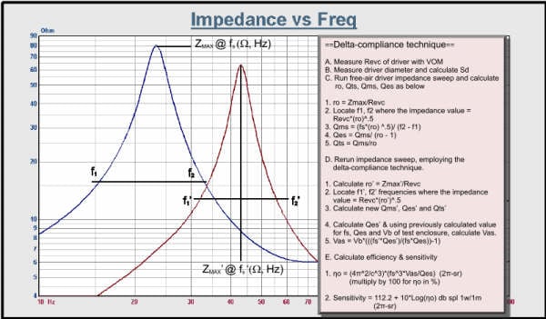
1a. System Impedance: Magnitude & Phase
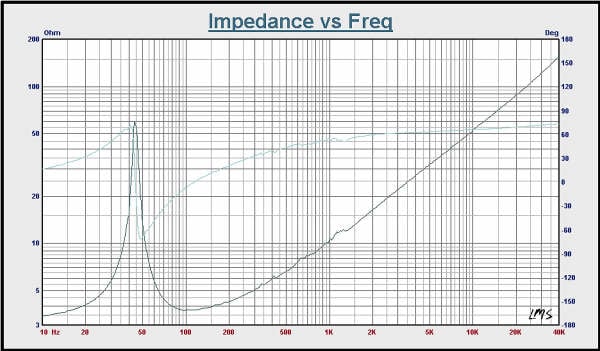
Figure 1: System Impedance
Purpose: To determine: (1) the characteristics of the impedance load
placed on a power amplifier by the system
across a defined frequency
spectrum segment; (2) various system parameters;
and (3) the identification of
any anomalies/pathologies that are reflected back to the electrical domain.
Value: Impedance curves provide an assessment of
the impedance the system presents to the driving
amplifier. When
presented with phase data it provides further insight into the
ease or difficulty
a given amp may face in driving
the system. Impedance curves also are useful in indicating
system parameters such as resonance frequencies,
system rated or nominal impedance
and so forth. In some cases, they can also provide evidence of a variety
of
system anomalies/pathologies, such as
pronounced standing-wave resonances arising within the air enclosed by
the cabinet.
Method of Measurement: Measure the driver’s Revc and the system’s
impedance (with driver still
in cabinet & any
internal power amp and/or processors disconnected from the driver), then remove the driver from
the cabinet and proceed to Section 2, Driver
Impedance, Magnitude & Phase. Except where it is noted otherwise or simply not
applicable, the suggested frequency spectrum is
10
Hz to 320 Hz.
For maximum accuracy, remove test lead and/or amp-to-sub cable impedance from all measured driver/system impedance curves. One method of accomplishing this is by measuring each beforehand and subtracting them from the driver/system measured impedance curve. Also, impedance measurements should be done in an environment as noise & vibration free as possible. Prior to making any acoustical or electrical measurements of the system, be sure to inspect all fittings, fixtures, hardware, etc to be certain that all are bolted down securely: leaks, loose hardware and so forth can and will effect measurement data.

Signal Used: Constant
voltage (preferred) or constant current, downward swept sine wave, MLS or impulse signal. Regarding the
swept sine wave, unless otherwise
required, use as low a test signal drive level as possible that can
repeatedly produce
clean data.
Metric Specification: Nominal or rated
impedance (Znom): should be stated such that the minimum impedance is no
less than 80% of the stated nominal or rated impedance.
Nominal System
Impedance, (10 – 320 Hz): A.A Ohms
Local minimum(s):
X.X Ohms (Mag. & Phase) @ Y.Y Hz
Local maximum(s):
W.W Ohms (Mag. & Phase) @ Z.Z Hz
1b. Driver Impedance: Magnitude & Phase
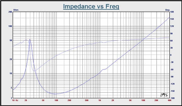
Figure 2: Driver Impedance
Purpose: To determine: (1) various driver/system parameters, and (2) the identification of any driver anomalies/pathologies reflected back to the electrical domain.
Value: Driver impedance curves provide for a great
deal of useful information, in addition to an assessment
of the
impedance presented by the system’s raw driver. Driver impedance curves are
useful for deriving Thiele-Small
parameters. In some cases, they
can also provide
evidence, as already mentioned of driver anomalies/pathologies
or other noteworthy characteristics.
Method of Measurement: Measure the driver’s Revc and the diameter of the driver, including
1/3rd to ½ the surround.
With
the driver out of the cabinet and secured in place or otherwise restrained from
any possible movement, remeasure the impedance. This is the driver free-air
impedance. Then using either the delta-mass (i.e., added-mass) or delta-compliance (i.e., added compliance) perturbation technique, remeasure the
driver’s impedance. From this and the previously taken free-air impedance
curve, derive the Thiele-Small parameter values. The change in mass or
compliance should be large enough so that the driver’s resonance frequency is
altered by at least 30%.
Signal Used: Constant voltage (preferred) or constant current, downward
swept sine wave, MLS or impulse signal. Unless otherwise required, use as low a test signal
drive level as possible that can repeatedly produce clean
data. Driver impedance measurements are measurement signal-level dependent
and the driver parameters derived from impedance measurements done at different
test signal levels will show differences.
Metric Specification: Driver T/S Parameter Table (See below).
 Σngineers
Note #1… Determining Raw Driver
Thiele/Small Parameters
Σngineers
Note #1… Determining Raw Driver
Thiele/Small Parameters
From
Measured Impedance Curves
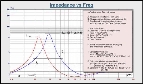
As expertly demonstrated by Thiele, Small, Benson, Novak and others, a great deal of useful information can be derived from a driver’s impedance curve. Collectively, the information gleaned from the raw data are formulated as defined parameters, a subset of which is commonly known as the “Thiele/Small” (T/S) parameters. Working up a small table populated with various T/S parameter values helps to round out the objective portion of a subwoofer assessment and provide a check against other measurements to ensure all around accuracy.
At left is an example of a commercially available speaker parameter utility at work. Two further graphics are presented each illustrating how to mathematically derive an estimate of a driver’s parameters from impedance data if you don’t have access to a program such as that shown at left. (See Bibliography ref. #38 in Part II for an in-depth discussion of both techniques)
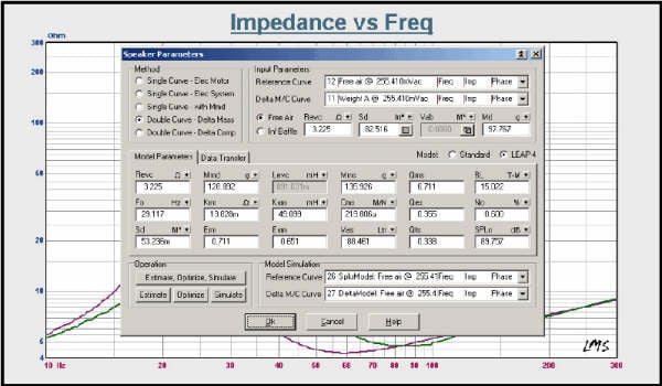
| PARAMETER |
VALUE |
| Revc (Ω) | 3.225 |
| fs (Hz) | 29.11 |
| Qts (-) | 0.338 |
| Vas (l) | 88.46 |
| Efficiency (%) | .600 |
| Sensitivity (dB/1W/1m) |
89.76 |
dB spl =
dBW + Sensitivity (dB) – 20* Log(D2/1m)
Where dBW = 10 *
Log(amplifier electric Watts out)
D2 = measurement
distance, meters
Complex, On-axis Frequency Response
2. Axial, Polar & Power Frequency Response; Sensitivity; Efficiency; Group Delay; Effective Frequency Bandwidth; Power Compression; and Maximum System Sound Pressure Level
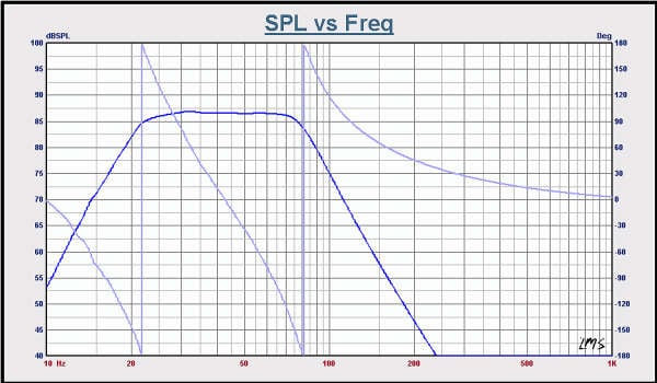
Figure 3: dB-SPL Plot
2a. Complex, On-axis frequency response.
Purpose: To determine the amplitude & phase response of the direct sound output of the subwoofer, across the frequency spectrum segment of interest.
Value: This gives us the actual amplitude & phase response of the subwoofer, free from the influence of the room. It’s a baseline that gives us a clear picture of the system’s actual performance.
Method of Measurement:
Near-field (Indoors): The measurement microphone should be placed such that it is centered on and normal to the dustcap. It should be positioned as close as possible to the surface of the dustcap, at its center point. This places the microphone at a reference point that is defined by the intersection of the reference axis and the reference plane. The axial amplitude-response measurement data produced by the microphone at this position is such that to all other frequency and directional-response amplitude response measurements are referred to it.
Keeping in mind the large displacements subwoofer driver diaphragms are capable of, the maximum excursion attainable should be determined beforehand, so as to prevent damage to either the driver or the microphone.
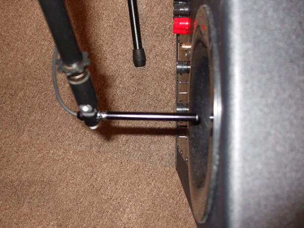
Figure 4a & b: Mic\Driver Disposition for NF Measurement. 4c: Mic\Port Disposition
Nearfield measurement can easily result in sound pressure levels in excess of that for which a particular measurement microphone might be rated. Prior to actual measurement, a series of test runs, using incrementally increasing drive levels, can be useful in establishing both driver excursion (as mentioned
above) & system sound pressure levels and how they relate to the measurement microphone’s rated SPL maximum. Overlaying a plot of the mic’s rated SPL maximum (red curve, above) prior to making any preliminary test measurements makes evaluation quick & easy. If measuring a ported system, establish maximum mic-safe system SPLs by measuring the port output first. And wear appropriate hearing protection!
Σngineers Note #2… Nearfield
Measurement: accuracy & limits;
Helpful hints & Tips
1. Keeping the measurement distance, r < 0.11a, where a = effective diameter of the driver being measured, keeps measurement errors to less than 1 dB of the true nearfield dB spl.
2. The theoretical upper frequency
(soft) limit for nearfield measurements is given
by:
(“soft”
as in various authorities quote either ka = 1 or ½; it can only be defined
loosely.)
ka = 1
Where:
k = wave number
a =
effective driver radius
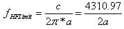
For radius, a, given in meters, the upper frequency limit is given by:
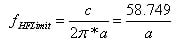
For radius given in cm, the upper frequency limit is given by:
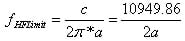
And for radius, a, given in inches:
If the subwoofer features a vented cabinet, the output of the duct(s) must be measured as well. As with the NF driver spl measurements, the measurement microphone should be placed such that it is centered on and normal to the center point of the duct’s external vent (Figure 4c). The individual amplitude response curves of all ducts are then scaled and vector summed with that of the driver(s) and the resulting system curve is then scaled to 1 meter. If the system curve data are scaled to a distance other than 1m, that should noted.
Multiple Drivers and/or Ports
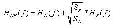
Where:
HNF(f) = System near-field response, dB spl
HD(f) = Driver near-field measured
response, dB spl
SP = Total effective radiating surface area of
the port(s), m2
SD =
Total effective radiating surface area of the driver(s), m2
HP(f) = Port near-field measured response,
dB spl
Method of Measurement:
Ground Plane (Outdoors): The subwoofer is placed on a solid, smooth surface in a position located well away from any other reflective boundaries. To ensure minimal acoustic interference (< 1dB contribution to total pressure) from objects large enough to be reflective at the wavelength of interest, the subwoofer should be located at a distance from said object or boundary that is no less than 5x the mic-to-cabinet measurement distance. The cabinet panel containing the driver(s) is then pointed at the microphone, positioned flush with the ground and located 2 meters along an imaginary axis, drawn from the center of the driver (for single driver systems) or center of the panel (for multiple-driver systems).
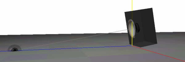
Figure 5: Ground Plane Measurement
In this arrangement, the microphone is measuring the combined amplitude response of the actual sub and a virtual or mirror image of the sub. In effect, the microphone is measuring the output of two identical sources, vibrating in phase and equal in strength - in a free field. With the mic sitting on the axis bisecting the sources, the on-axis pressure is doubled, the power generated has doubled, intensity has quadrupled and the sound pressure level is 6 dB up, compared to a sub measured free-field at the same distance.
If the system is driven with a 2.828 Vrms signal and measured at 2m using the ground plane approach, the resulting amplitude response plot will be virtually equivalent to that generated by the sub, at 1m, under free-field conditions, such as that obtaining at the top of a 100’ tower. System sensitivity can be determined from this plot and no magnitude scaling is required.
Suggested Nearfield & Groundplane Test Signal: Swept sine wave (320 Hz to 10 Hz), capturing sufficient data points to ensure post-processing accuracy, displayed on a semi-log plot, charting both magnitude and phase. The test signal is delivered at a pre-determined voltage, typically 2.828Vrms or calculated using 1W = V^2/Znom. For nearfield measurements, scaling the amplitude response plots to 1m, the sensitivity of the system can then be determined.
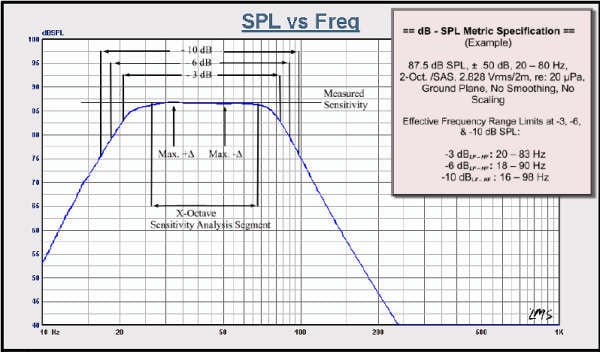 Sample complete dB – SPL Metric specification, without Sensitivity Analysis Segment (SAS).
87.5 dB SPL, ± .5 dB, 10 Hz to 320 Hz, 2.828Vrms/1m, re: 20 μPa, Near-field, On-axis, Scaled to 1m, No Smoothing, Swept Sine wave
-3dB lf/hf points: 20 – 83 Hz
-6dB lf/hf
points: 18 – 90 Hz
-10dB lf/hf points: 16 – 98 Hz
Max. deviation within -3 dB lf/hf points: +x, -y dB
== or ==
Complete dB – SPL Metric specification (with SAS)
87.5 dB SPL, ± .50 dB, 20 – 80 Hz, 2.828Vrms/1m,
re: 20 μPa, Near-field, On-axis, Scaled to 1m,
No Smoothing, Swept Sine Wave
(3-Oct. /S.A.S)
-3 dBLF – HF : 20 – 83 Hz
-6 dBLF – HF : 18 – 90 Hz
-10 dBLF – HF : 16 – 98 Hz
Max. deviation within -3 dB lf/hf points: +x, -y dB
Σngineers
Note #3… The far field: Where is it? How
do I know when my Mic is in it?
Key to any discussion concerning
the ground plane technique is the “far field” concept and how it applies to
microphone placement when measuring a subwoofer’s amplitude response.
In the far field of a subwoofer system, the subwoofer appears as a point source and sound pressure level varies inversely with distance, decreasing by 6 dB with each doubling of distance, or conversely, increasing by 6dB with each halving of distance.
Keeping this all this in mind, an expedient way to determine when a microphone has been placed in the far field is to simply run a series of amplitude response measurements, doubling the distance between the measurement mic and driver’s acoustic center (or other convenient reference point) and noting when the magnitude difference between plots, mid-band, reaches 6dB.
An old rule of thumb for estimating the far field boundary distance is to multiply the largest dimension of the source by 3. Note that with ground plane measurement, the “source” includes both actual and virtual sub.
2b. Polar response, Beamwidth, Directivity & Q.
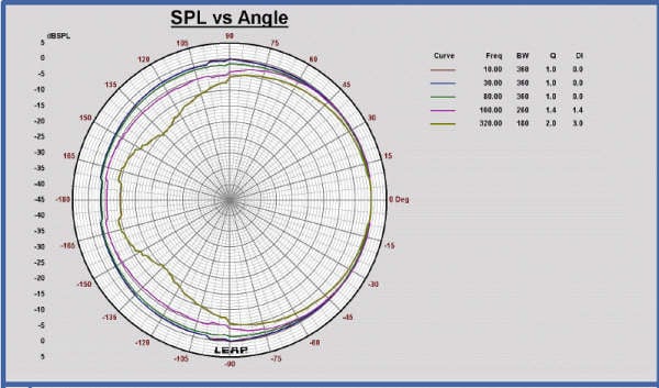
Figure 6: Polar response
Purpose: To determine the amplitude response of the subwoofer at various angles along a common plane, referenced to the on-axis amplitude response and measurement position.
Value: In addition to providing a wealth of information regarding the off-axis amplitude response characteristics of the subwoofer a variety of other performance specifications can be derived from the measurement data, such as beam width (BW), Q, directivity index (DI) and power response. Note that Q for directivity bears no relation to the quality factors Qms, Qes, and Qts. mentioned in Section 1b.
Method of Measurement: Ground-plane measurement lends itself particularly well to collecting polar response data as it requires only a bare minimum of hardware resources. Essentially, the sub is set up as for a standard on-axis measurement session. The reference point is established (the point of intersection between the reference axis with the reference plane) and the on-axis measurement is made. (If it is practical to raise the sub above the ground any response plot discrepancies owing to mutual coupling or baffle-size increase owing to actual-virtual system interaction can be minimized, however minimal they may be). The sub is then rotated, in angular increments, typically on the order of 5°, 10° or 15°. Below left shows a collection of such plots, in this case the measurements were made at 15° increments.
Once all the measurements have been collected, the curves are then normalized to the 0°on-axis curve by dividing each curve into the 0°on-axis curve. In doing so, the resulting plotted response at each point along the measurement path is relative to the on-axis response. Below right shows the result of normalizing the data plots at left. Though the data curves presented below right are normalized polar amplitude response curves, they are not usually presented in Cartesian format. Rather, they are more commonly seen as presented above in Figure 6.
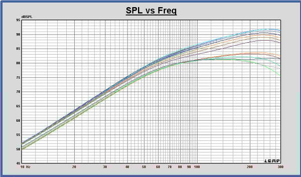
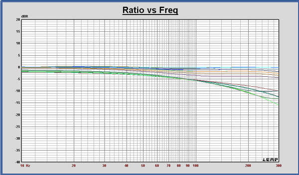
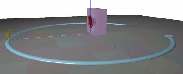
Figure 7: Horizontal plane polar response plot measurement layout
2b.II: Beam width (BW), Q, Directivity index (DI) and Power Response
Referring now to Figure 6, Beamwidth (also referred to as “coverage angle”) is that angle formed by drawing 2 radii, located either side of the reference axis, where the amplitude response, for a given frequency has decreased by 6dB, with respect to the 0° on-axis reference value. In Figure 6, the BW at 320 Hz is 180°.
Q is the numerical expression of the directionality of a system’s response. Strictly speaking, directivity is the ratio of axial intensity of the actual source to the intensity that would be produced by a point source emitting an equivalent amount of power. A source with equal output at a given frequency in every direction would have a Q = 1. With increasing directionality the Q value increases. A quick, first-order approximation of Q at a particular frequency (assuming axial symmetry) can be had by the following formula:
Q = 360°/BW°
where BW is specified in degrees.
The Directivity Index is simply the Q value specified above, expressed in dB. Specifically:
DI = 10 * Log (Q) (dB)
2c. Power response.
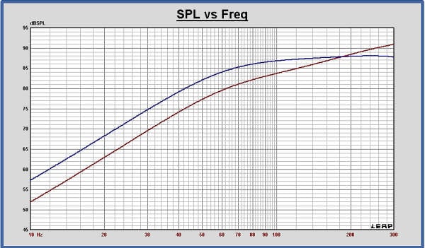
Figure 8: Red curve: system on-axis response; blue curve: system power response
Purpose: To determine
a subwoofer’s power response, expressed in dB spl.
Value: The axial amplitude response measurement, illustrated
in Section 2a, has traditionally been a mainstay of the objective assessment process. However, as important as
it is, it does not provide -in and of
itself - sufficient information to convey as complete a picture as is needed in
working up an
objective assessment of a subwoofer. Where the axial amplitude response
measurement resents
a view of the sub’s direct sound response characteristics as measured at a
single point in space, the power response gives an overall
view of the amplitude response characteristics of the sound field
generated by the sub, as measured at several points in space.
Method of Measurement: The approach here is similar to that for
capturing polar response data (see section 2b). And just as with polar response
measurement, groundplane measurement lends itself nicely to the power response
measurement process.
Common practice is to take measurements at 15° intervals, in both the horizontal (below, left) and vertical plane (below, right). (A common alternate is 15° intervals in the forward hemisphere, 30° intervals for the rear hemisphere; various factors may dictate less or more widely spaced intervals and measurement at intermediate angles). The resultant plots are then averaged to produce a good approximation of what is commonly referred to as the power response of the system.
2d. Sensitivity
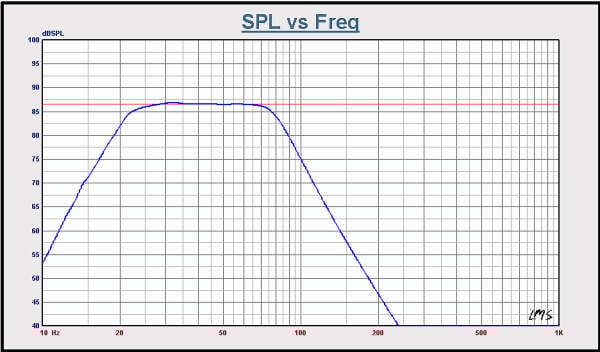
Figure 2: Sensitivity
Purpose: To determine the sound pressure level produced at 1m, on-axis, when 1 watt (power sensitivity) or 2.828 Vrms (voltage sensitivity) is applied to the subwoofer.
Value: Indicates the actual acoustical output, in
terms of sound pressure level, that will be produced by a
subwoofer, given an electrical input signal of a specified voltage or wattage,
the latter determined
by the nominal system impedance value (1W = V^2/Znom). Knowing a system’s sensitivity
assists in matching multiple systems. Also, dB-SPL acoustical output can be calculated given a
known amplifier wattage.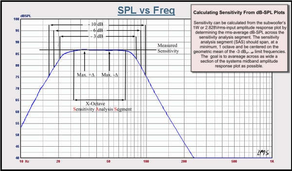
Approach: Sensitivity can be either measured or calculated (See Engineers Note #1 for the latter or graphic at right).
Signal Used: Swept sine wave (320 Hz to 10 Hz), capturing
sufficient data points to ensure post-processing accuracy, displayed on a semi-log plot, charting both
magnitude and phase. The test signal is delivered at a
pre-determined voltage, typically 2.828Vrms or calculated using 1W = V^2/Znom. Subsequently scaling the amplitude
response plots to 1m, the sensitivity of the system can then be determined.
Metric specification: XY dB spl, X-Oct averaged SAS, 1W or 2.828 Vrms/1m/4π/Znom
Σngineers Note #4… How do I calculate the
mid-band acoustic output of a sub if I know the sensitivity of the
unit, given a known electrical input, in Watts?
Where:
dB-SPL Out = Mid-band, On-axis, acoustical output at 1m
(dB-SPL)
Sensitivity = Measured or calculated sensitivity of the
device (dB-SPL)
W = Input electrical power (Watts)
Worked Example
The 1m, on-axis, sensitivity of a subwoofer is 87 dB - spl. The sub is a powered system and features an amplifier rated at 300 Watts. What is the mid-band, on-axis dB-SPL this sub can theoretically produce at 1m when fed an input at 300W?
dB-SPL Out = 87.50 dB-spl + 10 * Log(300.0)
dB-SPL Out = 112.1 dB-SPL, at 1m, On-axis, 2 –π SR
2e. Efficiency
Purpose: To determine the ratio of the acoustic power radiated by a subwoofer, PA, to the applied electrical power, PE.
Value: Electroacoustical efficiency indicates how much of the electrical power fed in to a subwoofer is converted into acoustical power radiated out. Usually expressed in % or dB, this metric is valid for the piston-band segment of the system’s pass band. It is a function of various T/S parameters and relates to sensitivity:
SP = 112.1 + 10*Log(η0) (dB SPL)
Approach : The subwoofers midband efficiency can calculated directly from the T/S parameters derived from the impedance measurements presented earlier. This equation assumes a radiation load of 2π-SR, free-field.
η0 = 100*(4π2/c2 * fs3Vas/Qes) (%)
η0 = 10*Log(4π2/c2 * fs3Vas/Qes) (dB)
Metric specification:
Efficiency (Half-space) = X.Y% or XX.Y dB
2f. Group Delay
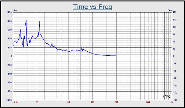
Figure 3: Group Delay
Purpose: To determine frequency-specific delay magnitude in terms of time for a given acoustic frequency band of interest.
Value: Group delay is the rate of change of the total phase shift with respect to angular frequency (the negative derivative of the phase function). Mathematically, it is expressed as:

In order that signal waveform fidelity may be preserved as it transits a given system, phase must change linearly with frequency response. Where phase nonlinearity exists, group delay exists.
Conversely, in a system where all frequencies transit in the same amount of time (or alternatively, transit with equal delay) no group delay exists. Time vs frequency Group delay plots indicate the degree of signal delay at any particular frequency.
Method of Measurement: Group delay is mathematically derived from the sub’s phase response by taking the negative derivative of the sub’s phase response with respect to frequency.
2g. Effective Frequency Bandwidth
Purpose: To determine the lower & upper frequency -3, -6, & -10 dB points, referenced to the subwoofers passband average dB SPL levels obtaining in the device’s maximum sensitivity zone.
Value: The EFB is useful for determining the passband of a device. The -3dB limits are given for comparative purposes, consistent with other published reviews. The -6dB limits are given to indicate the half-power points. The -10dB limits are chosen as they represent thedrop in dB spl levels sufficient to cause a perceived halving of the system’s output.
Approach: -3 dBLF – HF , -6 dBLF – HF , -10 dBLF – HF points are located with reference to the mid-band sensitivity level determined earlier. They are found at those frequency points at or external to the system’s passband. (See side graphics in Section 2a or 2b).
Metric specification:
-3 dBLF – HF : AA – BB Hz, re: mid-band sensitivity, XY dB
-6 dBLF
– HF : CC – DD Hz “ “
-10 dBLF – HF : EE – FF Hz “ “
[Presentation: -3 dBLF – HF, -6 dBLF – HF, -10 dBLF – HF == or == -3dBlf/hf, -6dBlf/hf, -10dBlf/hf]
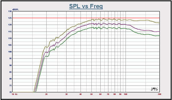
2h. Power Compression
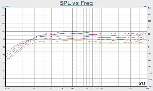
Figure 4: Power Compression
Purpose: To determine the degree to which a subwoofer’s otherwise linear input-output fundamental amplitude transfer characteristic becomes non-linear at increasing drive levels.
Value: Thermal effects (voice coil heating and a concomitant increase in voice coil resistance) along with various other driver nonlinearities seen arising in Bl(x), Le(x) and Cms(x) (force factor, inductance and compliance, respectively) and, of course, mechanical limitations all contrive to limit the acoustic output in such a way that it does not grow linearly with an increase in electrical input. Bl(x), Le(x) and Cms(x) are parameters treated, not as constants as when they are treated as small signal parameters but as quantities that vary with the excursion (x) of the voice coil from its rest position.
Power compression measurements give an assessment of the degree to which this nonlinearity presents itself, given a particular drive level. It also gives an indication of how well a subwoofer will accurately reproduce dynamic source material. Note: powered subwoofer systems often have limiter/compressor functions built into their processor algorithms to protect the driver(s) from possible damage. The effects of these limiter/compressor functions can appear similar in measurement to the results seen with a driver being driven hard enough for various nonlinearities to appear.
Approach: Near-field Approach (Indoors) or Ground Plane Approach (Outdoors)
Suggested Test Signal: Swept sine wave (320 Hz to 10 Hz), capturing sufficient data points to ensure post-processing accuracy, displayed on a semi-log plot and charting amplitude response. Beginning with a voltage drive level of 2.828 Vrms (or that calculated using 1W = V^2/Znom) the reference dB Spl curve is produced. The sweep is repeated, each time the input drive voltage is stepped in 1, 3, or 10 dB increments. Increase the drive voltage until 3dB worth of compression is noted. The resulting data can be displayed as either discrete curves (Figure 4) or if desired the curves can be normalized and scaled to the reference curve (Figure 5). Note: the slower the sweep the more noticeable will be thermal effects. An alternate signal useful for such testing is shaped pink noise as per IEC 268-1.
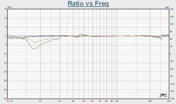
Figure 5: Power compression, curves normalized to the reference curve.
Metric Specification: 6 dB compression at ABC db-SPL amplitude magnitude, re: XYZ db drive voltage /1m/4π/Znom, XX Hz to YY Hz
Σngineers
Note #5… Homemade Wedge Micrometer
If you don’t want to rely on your
powers of estimation to size up maximum driver diaphragm displacement, a quick
means to determine maximum excursion is by use of a wedge micrometer.
2i. Maximum Sound Pressure Level
Purpose: To determine the maximum dB spl levels for which the device is capable, given power handling capabilities and system sensitivity. A calculated datum approximation that does not take into account power compression. Because it is based on the average passband sensitivity of the device, maximum dB spl is also an average value. For a measurement-based approach see CEA 2010 “ Standard Method of Measurement for Powered Subwoofers.”
Value: Useful for determining upper system output performance limits.
Approach: Given power capacity and average system
sensitivity, maximum sound pressure can be
calculated.
dB-SPL Out = Sensitivity + 10*Log(W) (dB-SPL)
Metric specification: dB-SPLMAX @ Rated Capacity (W or Vrms), 1m/Xπ-SR
Conclusion for Part I
Here in Part I of the Audioholics Subwoofer Measurement Protocol we’ve looked at a variety of measurements that, taken together, provide a good deal of insight regarding the performance characteristics of a subwoofer. Though the various topics presented illustrate a significant portion of the typical measurements approaches used today, the picture, nevertheless, remains incomplete. More information is needed to form an opinion of what any particular subwoofer will sound like than can be gleaned from the information presented by the various measurements illustrated in Part I.
In Part II we’ll take a look at things such as linear distortion, nonlinear distortion, mechanical noise, power amp performance characteristics (where applicable) and so forth. Ideally, with the objective data provided by the various measurement outlined in both Part I & 2, a reasonably accurate opinion of the subjective sonic qualities of the subwoofer can be formed.
Audioholics Subwoofer Measurement Protocol Bibliography
A.
1. Ahnert, Wolfgang, et. al.: “The Significance of Phase Data for the Acoustic Prediction of Combinations
of Sound Sources”, Audio Engineering Society Convention paper, 119th AES
Convention, Oct. 2005
2. Al-Ali, Khalid, Mohammad: “Loudspeakers: Modeling and Control”, UC Berkeley, Doctoral Dissertation,
1999
3. Allison, R. F. and Berkovitz, R.: “The Sound Field in Home Listening Rooms” Journal of the
Audio Engineering Society, Vol. 20, July/Aug. 1972
4. Aude, Arlo J.: “Audio Quality Measurement Primer” Application Note AN9789 Harris Semiconductor,
February 1998
B.
5. Benson, J E., “Theory & Design of Loudspeaker Enclosures”, Howard W. Sams & Co.,
Indianapolis, IN, 1996
6. Beranek, L. L.: “Acoustics”, McGraw-Hill, New York, N.Y., pg. 208, 1954.
7. J.M. Berman, J. M. et al.: “The Application of Digital Techniques to the Measurement
of Loudspeakers,” J. Audio Eng. Soc., Vol. 25, June 1977
8. Brüel & Kjær: “Basic Concepts of Sound”, Brüel & Kjær Lecture Note, English BA-7666-11, 1998
9. Brüel & Kjær: “Sound Intensity”, English BR 0476 – 14 Brüel & Kjær, Nærum, Denmark, Sept. 1993
10. Brüel & Kjær: “Basic Frequency Analysis of Sound”, Brüel & Kjær Lecture Note, English BA-7669-11, 1998
11. Brüel & Kjær: “Measuring Microphones”, Brüel & Kjær Lecture Note, English BA-7216-15,
Brüel & Kjær, Nærum, Denmark, May 1999
12. Brüel & Kjær: “Measurement Microphones, 2nd Edition”, English BR 0567 – 12
Brüel & Kjær, Nærum, Denmark, Aug. 1994
13. Brüel & Kjær: “Measuring Sound”, Brüel & Kjær, Nærum, Denmark, 198
14. Brüel & Kjær: “Microphone Handbook, Vol. 1: Theory”, Brüel & Kjær, English BE-1447 – 11
Nærum, Denmark, July 1996
15. Butler, Nathan: “Processor Setting Fundamentals”, Eastern Acoustic Works (EAW), Whitinsville, MA,
USA, Aug. 2001
16. Button, Douglas, J.: “A Loudspeaker Motor Structure for Very High Power Handling and High
Linear Excursion”, Audio Engineering Society, Preprint 2553, 83rd
Convention 1987
17. Button, Douglas, J.: “Heat Dissipation and Power Compression in Loudspeakers”, J. Audio
Eng. Soc., Audio Engineering Society, New York, N.Y., vol. 40, no. 1-2, Jan/Feb 1992
C.
18. Cable, C. R.: “Acoustics and the Active Enclosure,” J. Audio Eng Soc., Audio Engineering Society,
New York, N.Y., vol. 20, no. 10, 1972.
19. Cabot, Richard C.: “Fundamentals of Modern Audio Measurement”, J. Audio Eng Soc., Audio
Engineering Society, New York, N.Y., vol. 47, no. 9, 1999.
20. Cabot, Richard C., et. al.: “Time Domain Audio Measurements”,
21. Chau, K. H.-L., et. al.: “Measurement, Instrumentation and Sensors Handbook, Ch. 26: Pressure
and Sound Measurement”, CRC Press LLC, 2000
D.
22. Davis, Don: “Acoustic Attenuation With Increasing Distance”, Technical Letter # 218,
Altec Engineering News, Altec, Anaheim, CA
23. D’appolito, Dr. Joe: “Testing Loudspeakers” Audio Amateur Press, NH, USA, 1998
E.
24. Elko, Gary W., et. al.: “Room impulse response variation due to temperature fluctuations and its impact on
acoustic echo cancellation,” Avaya Labs, 2003
25. Engebretson, M. E.: “Directional Radiation Characteristics of Articulating Line Array
Loudspeaker Systems,” Audio Engineering Society Convention paper,
New York, November 2001,
F.
26. Farina, Angelo.: “Simultaeneous Measurement of Impulse Response and Distortion with a
Swept-Sine Technique”, Audio Engineering Society,Pre-print # 5093, AES 108th
Convention presentation, Feb. 2000
27. Fincham, L.R.: “Refinements in the Impulse Testing of Loudspeakers,” J. Audio Eng. Soc.,
Vol. 33, Mar. 1985
G.
28. Gander, M.: “Ground-Plane Acoustic Measurement of Loudspeaker Systems”, J. Audio Eng Soc., Audio
Engineering Society, New York, N.Y., vol. 30, no. 10, 1982.
29. Geddes, Earl R., “On Sound Radiation from Ported Enclosures”, Journal of the Audio Engineering
Society, Vol. 49, #3, March 2001
30. Griesinger, David: “Beyond MLS - Occupied hall measurement with FFT techniques”,
Lexicon, Waltham, MA, 1999
31. Gunness, D. W., et al.: “EAW Polar Measurements”, Eastern Acoustic Works (EAW), Whitinsville,
MA, USA, Sep. 2003
H.
32. Harris, Dr Steven, et. al.: “Personal Computer Audio Quality Measurements”, v. 1.00, Cirrus Logic
33. Henrickson, Clifford A.: “Directivity Response Of Single Direct-Radiator Loudspeakers In Enclosures”,
Technical Letter # 237, Altec Lansing Engineering Notes, Altec Lansing
Corporation, Anaheim, CA 1986
34. Henricksen, Clkifford A.: “Heat Transfer Mechanisms in Loudspeakers; Analysis, Measurement and Design.”
Audio Engineering Society, Preprint 2343, 80th AES Convention, 1986
I.
35. IEC: “Sound System Equipment Part 5: Loudspeakers”, 60268-5, International Electrotechnical
Commission, Geneva, Switzerland, 2001
36. IEC: “Sound System Equipment – Electroacoustical Transducers – Measurement of Large Signal
Parameters”, IEC – 100- 999, International Electrotechnical Commission, Geneva, Switzerland, 2005
37. IEC: “Electroacoustics – Sound level meters – Part 1: Specifications”, IEC 61672-1, International
Electrotechnical Commission, Geneva, Switzerland, 2002
38. IEC: “Sound System Equipment - Electroacoustical Transducers - Measurement of Large Signal
Parameters”, IEC 62458, International Electrotechnical Commission, Geneva, Switzerland
39. IEC: “Household high-fidelity audio equipment and systems – Methods of measuring and specifying
the performance – Part 5: Loudspeakers”, IEC 61305-5, International Electrotechnical
Commission, Geneva, Switzerland
40. IEC: “Electroacoustics – Sound level meters – Part 1: Specifications”, IEC 61672-1,
International Electrotechnical Commission, Geneva, Switzerland, 2002
J.
41. JBL, “Cinema Sound System Manual”, JBL Professional, Northridge, California, 2003
K.
42. Keele, D. B., “Development of Test Signals for the EIA-426-B Loudspeaker Power Rating Compact Disk”,
Audio Engineering Society Convention paper, 111th AES Convention, New York, Nov. 2001
43. Keele, D. B., “Anechoic Chamber Walls: Should They Be Resistive or Reactive at Low Frequencies”,
Journal of the Audio Engineering Society, Vol. 42, #6, June 1994
44. Keele, D.B.: “Low-Frequency Loudspeaker Assessment by Near-field Sound Pressure Measurement”
J. Audio Eng Soc., Audio Engineering Society, New York, N.Y., vol. 22, no. 4, 1974.
45. Keele, D.B.: “Maximum Efficiency of Direct-Radiator Loudspeakers” Pre-print 3193
Audio Engineering Society Convention paper, 91st AES Convention, New York, Oct. 1991.
46. Keele, D.B.: “A New Set of Sixth-Order Vented-Box Loudspeaker System Alignments” Pre-print 3193
J. Audio Eng Soc., Audio Engineering Society, New York, N.Y., vol. 23, no. 5, Jun., 1975
47. Keele, D.B.: “Time-Frequency Display of Electro-Acoustic Data Using Cycle-Octave Wavelet Transforms”
Pre-print 4136, Audio Engineering Society Convention paper, 99th AES Convention,
New York, Oct. 1995
48. Kelloniemi, Antti et al.: “Detection of subwoofer depending on crossover frequency and spatial
angle between subwoofer and main speaker” Convention paper 6431,
Audio Engineering Society Convention paper, 118th AES Convention,
Barcelona, Spain May 2005
49. Khenkin, Alex.: "How Earthworks Measures Microphones", Earthworks, No Date Given
50. Klapman, S. J., “Interaction Impedance of a System of Circular Pistons”, Journal of the Audio Society
of America, January 1940
51. Klippel, Wolfgang: “Assessment of Voice Coil Peak Displacement Xmax”, Audio Engineering Society
Convention paper, 112th AES Convention, München, May 2002
52. Klippel, Wolfgang: “Loudspeaker Nonlinearities – Causes, Parameters, Symptoms”,
Audio Engineering Society Convention paper, 110th AES Convention, Amsterdam,
May 2002
L.
53. Li, Aijun, et. al.: “The Problem of Offset in Measurements Made Using Acoustic Pulse Reflectometry”,
Acta Acustica United With Acustica, Vol. 91 S. Hirzel Verlag (2005)
M.
54. Mateljan, Ivo, et. al.: “The Comparison of Room Impulse Response Measuring Systems”, University of
Split, Croatia, 2003
55. McGregor, Chuck, “Community Data Measurements”, Community Professional Loudspeakers,
Chester, Pennsylvania, USA
56. Mayr, H.: “Theory of Vented Loudspeaker Enclosures,” J. Audio Eng Soc., Audio Engineering
Society, New York, N.Y., vol. 53, no. 2, pg. 91, 1984.
57. McKnight, J., Woodgate, J.M., et. al.: “AES project report for articles on professional audio and for
equipment specifications — Notations for expressing levels”,
AES R2-2004, Audio Engineering Society, New York 2004
58. Miller, Robert E. et al.: “Physiological and content considerations for a second low frequency channel
for bass management, subwoofers, and LFE” Audio Engineering Society
Convention paper 6628, 119th AES Convention, NY, NY, USA, October 2005
59. Mowry, Steve: “Loudspeakers and Magnets et al”, SM Audio Engineering Consulting, September 2004
60. Mowry, Steve: “Transducer Design Using 2D FEA & BEM”, SM Audio Engineering Consulting, 2003
61. Muller, Sven and Massarani, Paolo: ”Transfer-Function Measurement with Sweeps: Director’s Cut Including
Previously Unreleased Material”
N.
62. National Instruments: “Measurement Encyclopedia: Acoustics, Measurements”, National Instruments,
2005
63. National Instruments: “Measurement Encyclopedia: Hardware, Acoustic Test Chambers and
Environments”, National Instruments, 2005
64. Newman, R. J.: “A. N. Thiel, Sage of Vented Speakers,” Audio, August 1975.
65. Noselli, Guido: “Parametri sintetici per la valutazione d'un impianto audio professionale per il rinforzo
del suono”. 1a parte, (Concise Parameters For Assessing A Pro Audio System For Sound
Reinforcement Use, Part 1), Sound & Lite, January 2001
66. Noselli, Guido: “Parametri sintetici per la valutazione d'un impianto audio professionale per il rinforzo
del suono”. 2a parte, (Concise Parameters For Assessing A Pro Audio System For Sound
Reinforcement Use, Part 2), Sound & Lite, March 2001
67. Noselli, Guido: “Parametri sintetici per la valutazione d'un impianto audio professionale per il rinforzo
del suono”. 3a parte, (Concise Parameters For Assessing A Pro Audio System For Sound
Reinforcement Use, Part 3), Sound & Lite, May 2001
O.
68. Ole-Herman, Bjor: “Measurement of Extremely Low Sound Pressure Levels”, Norsonic Application
Note, Norsonic AS, Lierskargen, Norway, 1999
69. Olson, H. F.: Elements of Acoustical Engineering, Van Nostrand, Princeton, N.J., pg. 148., 1957.
70. Olson, H. F.: “Direct Radiator Loudspeaker Enclosures,” J. Audio Eng Soc., Audio Engineering
Society, New York, N.Y., vol. 17, no. 1, pg. 22, 1969.
P.
71. Penkov, G., et al.: “Closed-Box Loudspeaker Systems Equalization and Power Requirements,” J.
Audio Eng Soc., Audio Engineering Society, New York, N.Y., vol. 33, no. 6, pg. 447, 1985.
72. Phillips, Alan S.: “Measuring the True Acoustical Response of Loudspeakers” SAE Technical Paper,
2004-01-1694, SAE, Warrendale, PA, USA, 2004
Q.
R.
73. Rasmussen, Per: “Measurement, Instrumentation and Sensors Handbook, Ch. 27:
Acoustic Measurement”, CRC Press LLC, 2000
74. Russell, David A., et al.: “Acoustic monopoles, dipoles, and quadrupoles: An experiment revisited”
American Journal of Physics, August 1999
S.
75. Sakamoto, N.: “Loudspeaker and Loudspeaker System”s, Nikkan Kogyo Shinbunshya, pg. 101,
1967 (in Japanese).
76. Shust, Michael, R., et. al: “Electronic Removal of Outdoor Microphone Wind Noise”,
Acoustical Society of America, Paper 2pSPb3, presented 136th
ASA meeting, October 1998
77. Simmons, Dan: “Uncertainty due to boundary reflections” National Physical Laboratory,
Middlesex, UK, 2004
78. Small, R. H.: “Direct-Radiator Loudspeaker System Analysis”, J. Audio Eng Soc., Audio Engineering
Society, New York, N.Y., vol. 20, June, 1972.
79. Small, R. H.: “Closed-Box Loudspeaker Systems, Part 1: Analysis”, J. Audio Eng Soc., Audio Engineering
Society, New York, N.Y., vol. 20, no. 10, 1972.
80. Small, R. H.: “Vented-Box Loudspeaker Systems, Part 1: Small-signal Analysis”, J. Audio Eng Soc., Audio
Engineering Society, New York, N.Y., vol. 21, no. 6, 1973.
81. Staffeldt, Henrik: “Acoustic Center or Time Origin ?”, Department of Applied Electronics, Technical
University of Denmark, Lyngby, Denmark, 1998
82. Starobin, Brad: “CEA-2010: Standard Method of Measurement for Powered Subwoofers”,
Consumer Electronics Association, Jan. 2006
83. Struck, Christopher J., Temme, Steve F.: “A Comparison Of Techniques For Evaluation Of Loudspeaker
Performance at Low Frequencies”, Brüel & Kjær, Nærum,
Denmark
84. Struck, Christopher J., Temme, Steve F.: “Simulated Free Field Measurements”, Audio
Engineering Society, Pre-print # 3397, AES 93rd
Convention presentation, Oct. 1992
T.
85. Temme, Steve F., “Are you Shipping Defective Loudspeakers to Your Customers ?”, Listen, Inc.,
Boston, MA, USA
86. Thiele, A. N., “Loudspeakers in Vented Boxes”, Journal of the Audio Engineering Society, Vol. 19,
May 1971
87. Thiele, A. N., “Estimating the Loudspeaker Response when the Vent Output is Delayed”,
Journal of the Audio Engineering Society, Vol. 50, #3, May 2002
U.
V.
88. Various Authors, “AES Recommended Practice Specification of Loudspeaker Components Used
in Professional Audio and Sound Reinforcement”, Audio Engineering
Society, AES2-1984 (r2003), New York, 2003
89. Various Authors, “System Specification Standard”, Eastern Acoustic Works (EAW), RD0069, Rev 008,
Sept. 2003
90. Various Authors, “Specification Sheet Details”, Eastern Acoustic Works (EAW), Whitinsville, MA,
USA, Sept. 2003
91. Various Authors, “Home THX Audio System Room Equalization Manual”, Rev. 1.5, Lucasfilm, Ltd.,
1996
92. Various Authors, “Notations for expressing levels”, AES Project Report, AES R2-2004,
Audio Engineering Society, NY, NY, USA, 2004
93. Various Authors, “Useful Equations For The Sound Contractor”, Technical Letter #166
Altec Lansing Engineering Notes, Anaheim, CA
94. Various Authors, “Decibels”, Technical Letter #212A
Altec Lansing Engineering News, Anaheim, CA
95. Vassilis, Tsakiris et al.: “Optimum Loudspeaker System with Subwoofer and Digital Equalization”
Audio Engineering Society Convention paper, 117th AES Convention,
San Francisco, CA, USA, October 2004
96. Voishvillo, Alex: “Assessment of Loudspeaker Large Signal Performance – Comparison of
Different Testing Methods”, Audio Engineering Society Convention paper,
111th AES Convention, New York, November 2001
W.
97. Wagner, Randall, et al.: “Determination of acoustic center correction values for type LS2aP
microphones at normal incidence”, Journal of the Acoustical Society
of America, Jul. 1998
98. Woolf, Chris, “How to reduce wind noise and vibration”, Rycote Microphone Windshields Ltd, 2002
X.
Y.
Z.