
Understanding Loudspeaker Review Measurements Part II
image courtesy of Dayton Audio
Frequency Response Waterfall Plots
One way that Audioholics have presented on-axis and off-axis frequency responses in our loudspeaker reviews are through waterfall plots.
Wikipedia defines a waterfall plot as:
“a three-dimensional plot in which multiple curves of data, typically spectra, are displayed simultaneously. Typically the curves are staggered both across the screen and vertically, with 'nearer' curves masking the ones behind.”
This is a great way to show the frequency responses over the entirety of an axis because so much information can be conveyed in such an intuitive way. Waterfall plots can give the viewer an immediate sense of the linearity of the loudspeaker over a large angle of its coverage. They also let the viewer know how directional the speaker is at a glance. However, they are not a customary look at a loudspeaker’s frequency response, and that can make them somewhat puzzling for those people expecting a traditional frequency response. In this article, we hope to disentangle these graphs so that anyone can easily understand the significance and nature of the information that they contain. We will also be looking at polar maps since they cover the same information from a different but also illuminating perspective.
One thing to note before continuing to discuss frequency response waterfall plots is that these are NOT the same as the waterfall graphs that Room EQ Wizard generates. The waterfall graphs generated by Room EQ Wizard do not show responses at differing angles; instead, they use time progression on the x-axis. Room EQ Wizard’s waterfall graphs show how long it takes for sound to decay per frequency, but this is NOT what is being displayed in Audioholic’s waterfall graphs in our loudspeaker reviews at all.
At Audioholics, we typically show frequency response waterfall plots in a profile view and also a diagonal view. The profile view more easily allows the viewer to see the response shape of each individual curve. The diagonal view is better at giving those curves more context regarding their specific angle. In other words, the diagonal view is better to see how much the response is changing as the measurements move further off-axis. The profile view is a two-dimensional view, since it only shows two axes of the measurements, and the diagonal view is, of course, a three-dimensional view since we see three axes.
While the waterfall plots are a relatively accessible way to look at the frequency response over an axis of a speaker, it is still a lot of information to digest for someone who is not accustomed to seeing response data presented like this. For this reason, we are going to illustrate what is occurring one step at a time. First, let’s take a look at what the on-axis frequency response alone looks like in these plots. In the below examples, we will use real measurements from our Outlaw Audio BLSv2 review. The reason why we chose the BLSv2 speaker is because it is a fairly typical, well-rounded loudspeaker that has conventionally good characteristics.
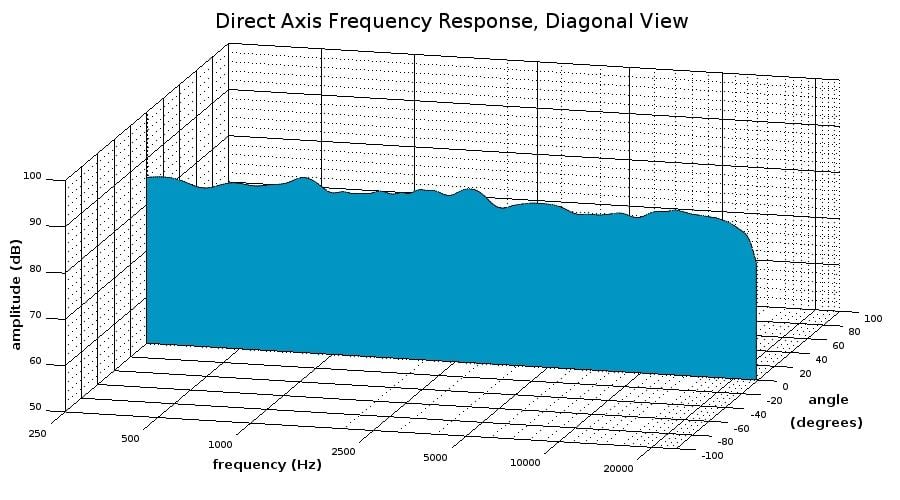
Diagonal view of a waterfall plot showing the on-axis response only
Note that in the above diagonal view of our waterfall plot, we see the on-axis response is placed squarely in the center of this box at zero degrees in the angle axis because the on-axis response is almost always going to be the most important curve in this set. The on-axis response is usually going to be the angle at which the speaker emits the most acoustic energy, so it is normally higher in amplitude on average than off-axis angles.
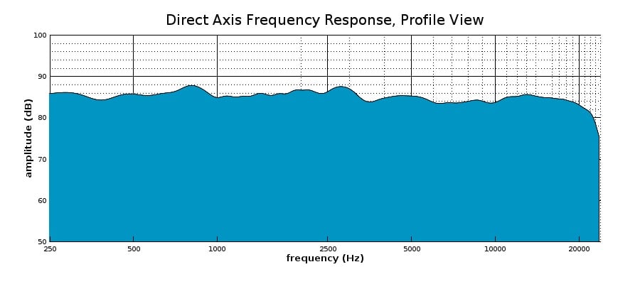
Profile view of a waterfall graph showing the on-axis response only
In the profile view, we don’t see the angle, but we get a better sense of the shape of the response.
Now let’s look at the on-axis response along with the response at 90-degrees. Of course, the 90-degree angle is perpendicular to the on-axis angle, so it will be the speaker’s frequency response at a right angle to the side of the speaker.
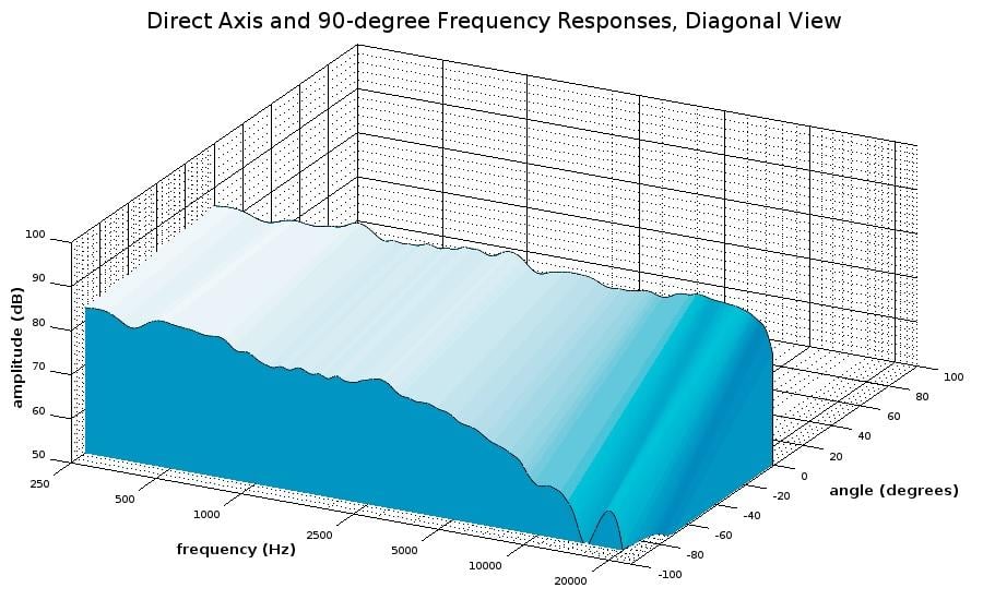
Diagonal view of a waterfall plot showing the on-axis response and 90-degree response
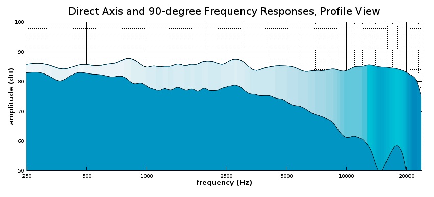
Profile view of a waterfall plot showing the on-axis response and 90-degree response
One thing to note is that we have added a surface that stretches over the two curves so that it is easy to see the gradient of change between them. As expected, the 90-degree angle response is considerably lower in amplitude than the on-axis response, especially as we move up in frequency. Most direct-radiator speakers (with only forward-facing drivers, which is most conventional speakers) show some version of this behavior where the higher frequencies lose energy more rapidly as the angle moves farther away from the direct on-axis angle. The problem with showing just the on-axis response and 90-degree response is that we don’t see much resolution in between those angles. Let’s throw in a 45-degree angle to get a better sense of what is happening between this wide angle:
Diagonal view of a waterfall plot showing the on-axis, 45-degree, and 90-degree responses

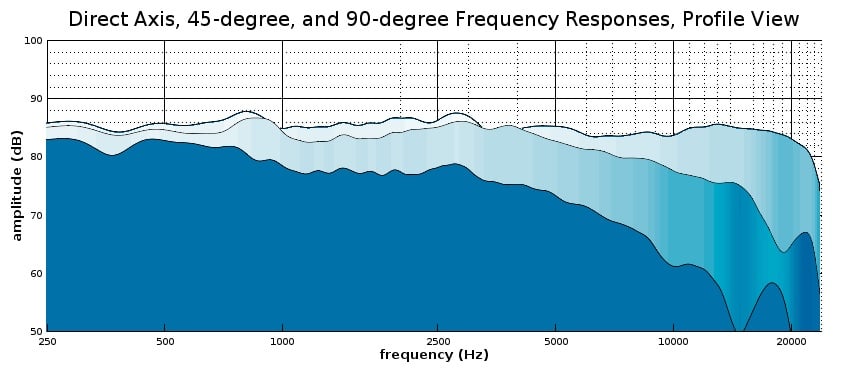
Profile view of a waterfall plot showing the on-axis response, 45-degree, and 90-degree response
With the addition of the 45-degree measurement, we get a better understanding of their speaker’s behavior within its front hemisphere, and what’s more, 45-degrees is a much more pertinent angle than 90-degrees since few people will be listening to the speaker at a right angle to the front of it. We can see that at 45-degrees, the speaker holds nearly the same level of amplitude until around 4 kHz where it begins to roll off at a gradual rate. This gradual roll off takes a steeper turn at around 15 kHz, so those who want to hear high treble frequencies from this speaker should be listening at a much closer angle to its front axis than 45-degrees.
While we can tell a lot more about this speaker’s dispersion with the inclusion of the 45-degree angle, it still isn’t a very detailed look at its overall off-axis response. Let’s fill in all of these angles at 10-degree increments. That will give us a very good view of how this speaker behaves off-axis. Let’s also expand this plot to include the other half of these angles so we get a better sense of the overall shape of this speaker’s dispersion:
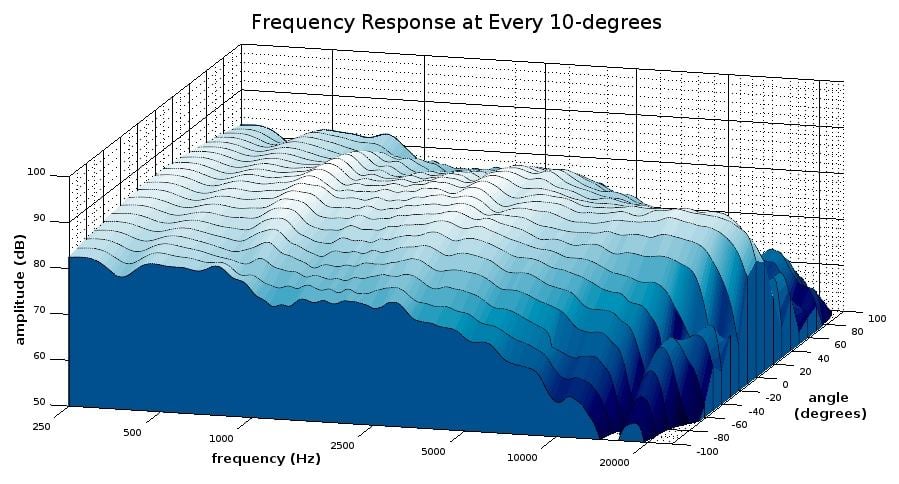
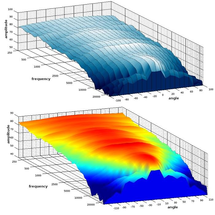
Diagonal view of a waterfall plot showing all responses in 10-degree increments out to 100-degrees
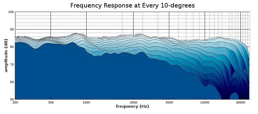
Profile view of a waterfall plot showing all responses in 10-degree increments out to 100-degrees
One advantage of this more comprehensive look at the speaker’s off-axis responses is that we can see at what angle the upper treble really drops off. This is useful for determining at what angle this speaker will still provide a tonally ‘full’ sound. From observing these graphs, it looks like the upper treble on this speaker takes a big tumble at the 40-degree angle and outward, so those who want to hear a full range of sound should listen within a 30-degree angle of the front axis. That constitutes a 60-degree angle over the front of the speaker, so that should be pretty easy to achieve in any normal listening situation. However, even if one listens a bit further off-axis than that, high-frequencies do get reflected in the reverberant field, which is to say a normal listening position in-room, so, in practice, a listener can still get more exposure to higher levels of high frequencies than that off-axis roll-off indicates.
Something else that is useful from examining waterfall plots like this is that, from seeing how much of the high frequencies are attenuated as we move farther from the on-axis angle, we can choose which axis response fits our preferences better. For example, this speaker may be a bit bright for some people’s tastes if listened to on-axis, but the 20-degree angle tones down the treble response without losing it entirely. Using the 20-degree angle as the direct listening axis can give this speaker a warmer character for those who prefer that. The angle at which you listen to your speakers can often act as a tone control, and these waterfall plots let you know what kind of responses different angles can yield. Some speakers are not intended to be listened on-axis, and waterfall plots can give you an idea of the angle at which they might sound better.
In Audioholics’ loudspeaker reviews, we use a white-blue color map to denote when the waterfall plot depicts the responses on a horizontal axis. For the vertical axis, we use a blue-green color map for waterfall plots depicting the responses of a vertical axis. We decided on a blue-green color scheme for the vertical plots because it looks cool, but we also wanted them to be easily differentiated from the horizontal response graphs. As we always note in our reviews, the response of the vertical axis isn’t nearly as important as the speaker’s behavior in the horizontal axis, so don’t be alarmed if the vertical off-axis behavior in a loudspeaker gets pretty ragged. What should be looked at in the vertical waterfall plots is how narrow of an angle that an even response occurs around the on-axis angle. If the speaker only bears a smoothish response at the on-axis angle, then the speaker should be listened with the ears level with the speaker, and usually at the tweeter. If the angles around the on-axis angle have a similarly smooth response, then it isn’t as critical that the speaker is listened to with ears at the same level.
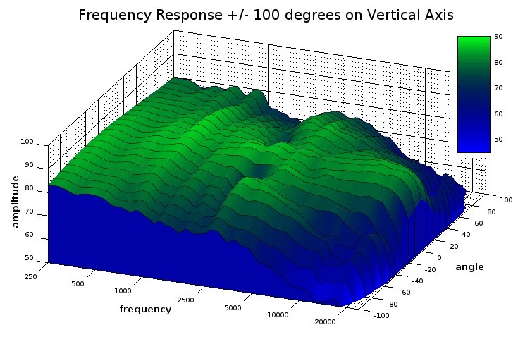
Diagonal view of a waterfall plot showing all responses in 10-degree increments out to 100-degrees on the vertical axis
Polar Maps
Another type of plot that readers will see in Audioholics’ reviews is the polar map (sometimes it is also referred to as a directivity sonogram). A polar map shows the same information as the waterfall plots, but they show that data from a different perspective. It is a ‘top-down’ view of the frequency response over an angle of measurements, and since it loses the amplitude axis in such a perspective, it is a two-dimensional view. Instead of using an axis to represent amplitude, the polar map uses color; warmer colors signify greater amplitude. To illustrate the relationship between the waterfall graph and the polar map, let’s take a diagonal look at both of them using the same measurement set for comparison:
Diagonal view of a waterfall plot and diagonal view of a polar map.
What can be seen in the above graph is that the polar map basically just gives the waterfall plots a new paint job. While it is interesting to view the polar map from a diagonal view, it is much more useful to look at it from the top-down view:
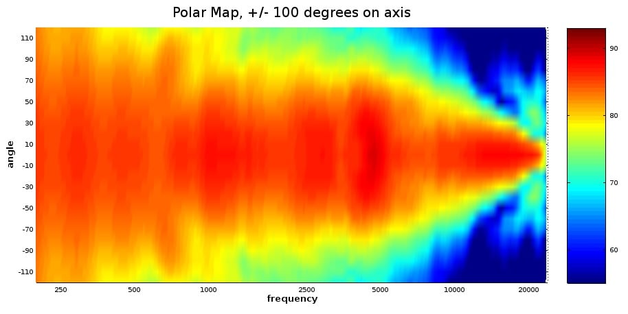
Polar map - top-down view.
In this top-down view, we get a very good look at the broader trends in the speaker’s dispersion pattern. Areas where the color is a solid and consistent red hue should have a full and balanced sound. We can see, from the example above, that speaker has a relatively even coverage pattern up to roughly 6 kHz, where the dispersion begins to contract at higher frequencies. This is not necessarily a bad quality; this speaker should have a tonally balanced sound around the on-axis angle, but those who want a warmer sound where the treble is toned down just a bit can listen to this speaker at an angle where the treble is partially rolled off, like the 40-degree angle for example. Ideally, what we want to look for is uniform coverage per angle, so that the speaker’s character does not change according to angle. Something like the following graph would be an ideal:
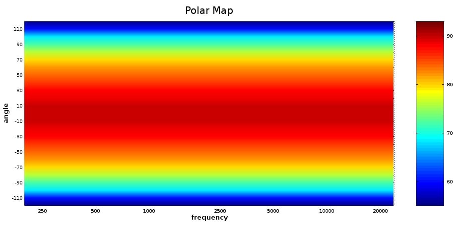
Polar map Ideal.
The above example is, of course, an impossibility in reality. However, it does illustrate a kind of directivity control to which loudspeakers should be striving. But speakers that do not meet that perfect behavior are not necessarily bad. Consider the graph up above our ideal where the treble contracts above 6 kHz; that contracted treble can be used to the advantage of listener’s preference. Something else to consider is that no conventional speaker can control the directivity in low-frequencies, but the acoustic effects of that characteristic won’t necessarily be heard as a flaw (it is for this reason we don’t do directivity tests for subwoofer--they are all omnidirectional in their intended frequency range use). Furthermore, what is sometimes seen as a major flaw in a plot of measurements can be difficult to hear in actuality. In some ways, human hearing is very acute to flaws in sound reproduction, but in other ways, human hearing can be very insensitive to problems that can be seen in measurements. I have heard plenty of speakers that have had a multitude of measured problems. Yet, I still thought they sounded good. One such case is the below graph:
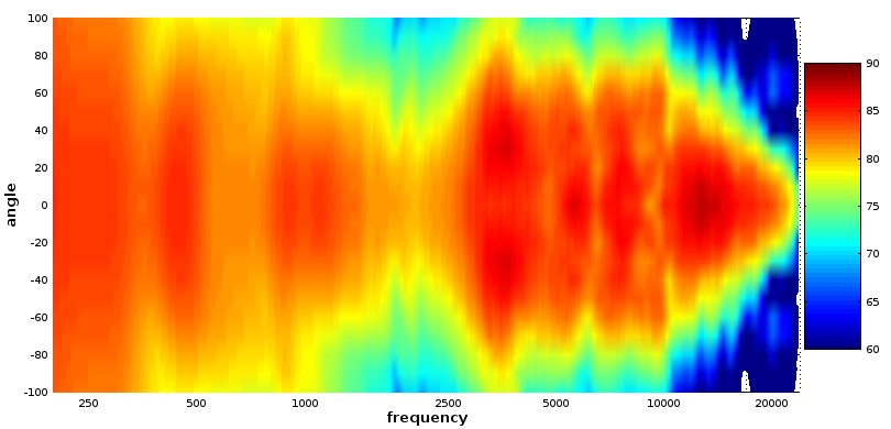
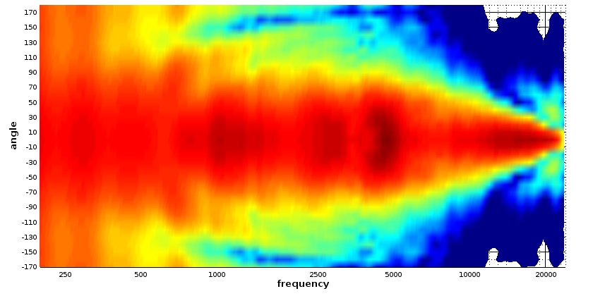
Not ideal polar map - can you spot the flaw?
The above speaker exhibits a very significant constriction in directivity centered around 2 kHz. Yet, in my opinion, this speaker did not sound bad, and I enjoyed them. It may be that if it were played back to back against a speaker that had superior directivity control in this region, the problem would become more evident. Indeed, if one were listening outside of a 40-degree angle, I would expect this flaw to be much more glaring, but with it positioned on-axis, I didn’t get a sense that anything serious was missing.
Perhaps a more intuitive way to look at a polar map is to put it in a radial plot because this is analogously closer to how the speaker actually behaves. The above polar maps place all the angles in a Cartesian grid, but that is an extra level of abstraction done to make certain features easier to examine. A radial plot, on the other hand, looks at the angles according to how they were actually measured with respect to the speaker. Here are the same measurements used in the above Cartesian polar maps, now mapped in a radial plot:
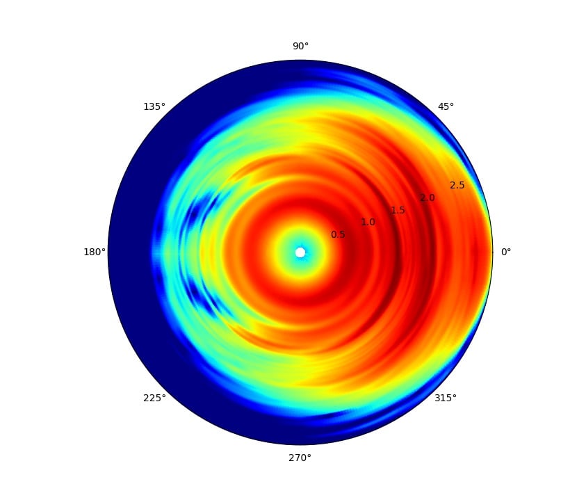
Polar map of a radial plot
While radial plots are, in a sense, a more ‘true’ manner of displaying the speaker’s dispersion, it is a bit more difficult to make out details and gauge their significance. Laying out the polar map in a Cartesian grid is much easier to understand key features of the measurement set at a glance. For this reason, we display the polar maps in a grid rather than a radial plot.
Now, for those who are curious, let’s take a look at what our perfectly uniform dispersion speaker would look like in a radial graph, the "Polar Map Ideal" example from a couple of graphs above:
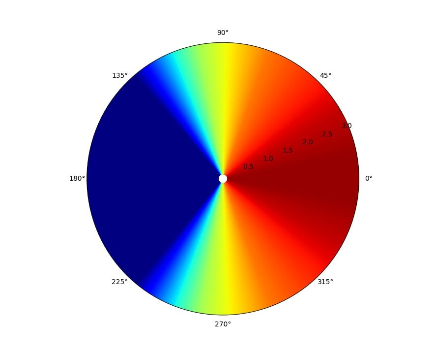
Polar map of a radial plot from an imaginary speaker with a perfectly uniform dispersion
Note that these radial plots cover the entire 360 degrees of the speaker’s circumference. We can show that data in our Cartesian graphs. The rear semicircle of the speaker’s output is not normally an important metric (except perhaps in dipole speaker designs), so we typically omit depicting those measurements. For the curious, here is what that full 360-degree measurement set looks like in a Cartesian grid:
Polar map showing full circumference of angles
In the above graph, showing the full 360 degrees of a loudspeaker in a Cartesian grid, one obvious feature that we see is that the high frequencies beam in a very narrow angle while the low frequencies look to project sound outward in every direction at about the same loudness level. It should be kept in mind that the top and bottom of that 360-degree graph represent the rear of the loudspeaker. The high-frequency energy is so contained at the top end that the recorded output drops below the exhibited amplitude range at angles opposite of direct axis and so leaves a small blank area in the high-frequency graphs. The obvious lesson here is that if you want to hear high-frequencies from this speaker, you must be listening in front of it, not behind it.
Conclusion
Hopefully, this article has given readers a deeper appreciation for the contents of these graphs. They are more than just pretty pictures. They are a map of the behavior of the measured loudspeakers and can serve as a great guide in not only ascertaining the sound character of the speaker, but also for determining the best positioning and placement manipulation to get the best sound out of them.
Please revisit: Understanding Loudspeaker Review Measurements Part I where we discuss on and off-axis frequency response, directivity index and more. In Part III, the final installment of this series, we discuss subwoofer distortion measurements.
James Larson is Audioholics' primary loudspeaker and subwoofer reviewer on account of his deep knowledge of loudspeaker functioning and performance and also his overall enthusiasm toward moving the state of audio science forward.
View full profile