Acoustical Measurements - What are They?

In this second article we want to continue to build some fundamentals that will be very important in understanding what could be wrong with the listening room and ultimately: how can I fix the listening room. I have heard some people claim "I just listen and walk around the room and clap my hands and I know what to do." I would say this is another "myth". What is true, is that final tuning of a room often does require extensive and subjective listening. But to get one in the ball park, you will need basic measurements.

In this article we will discuss Frequency Response, Reverberation Time, Energy Time Curves, Waterfall plots, and the much debated Psycho-acoustical Response Curves.

Frequency Response.

Our original definition was pretty simple, it's the frequency within the human hearing range, namely 20Hz to 20kHz. So what would the goal be? A flat frequency response from 20Hz to 20kHz, right? Maybe. It depends on how it's being measured and there are also subjective preferences. First off, what is a flat frequency response? Sounds like a simple question, but have you thought it through. On a linear frequency scale you probably would not like the sound of a flat frequency response. It would be rather bright. Our hearing is logarithmic. We generally graph frequency response on a logarithmic scale. In this context a linear, or near linear frequency response would be desired. Now, while this article is not about taking measurements (that's for next month), let's quickly look at "white noise" vs "pink noise". White noise is the noise that which, in a perfectly responding system would, give you a flat frequency response when you graph the response on a linear scale. Pink noise is more often used, as its goal is a flat response on a logarithmic scale. Since the later is what we strive for, almost no one uses white noise generators anymore.

Here is a graph of a linear frequency response. You will note how jagged it is, but that should not be a cause for alarm. This is normal comb filtering that occurs in almost all listening rooms. What is interesting to note is that overall the response is gently sloping down, decaying. Thus there's a little more energy at the lower octaves relative to the higher octaves.

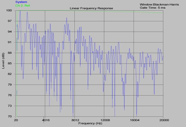
The second part I mentioned was about goals or our subjective preferences. What do we want? Do we always want flat?

The human ear is not flat. By that I mean that we do not hear every frequency at the same volume. Simply put, the human ear and the brain to which it connects is designed with a primary goal in mind: to reproduce and interpret speech. This means that there is a narrow band of frequencies that we hear more clearly than we hear others. The generally accepted range of these 'speech' frequencies is between 500Hz and 5Khz. Because of this phenomena we do not hear the upper and lower registers of the 20-20,000 cycles bandwidth as easily. Because of this, most people actually don't subjectively want a flat frequency response. Also, because lower frequencies are harder to hear at lower levels, most people like a little added in the bottom end and, in many cases, gently tapering off as one gets into the upper octaves. If you've heard a system that you really subjectively liked, it would be interesting to measure it and see how flat it really was. Conversely, we've had clients that knew that their hearing in the higher octaves was not as good as it used to be. We've actually designed rooms that allow for more of the energy (and recommended speakers that excel) in the higher octaves. Some people would potentially frown on this approach, but music is ultimately for enjoyment, not the statistics of measurements. They should be used as information and tools to get us to that level of enjoyment, but not dictate what enjoyment is.

Reverberation time.

This is the time it takes for an initial sound to decay a certain number of decibels. The technical definition of RT-60, or Reverberation Time, the time that it takes a sound to decay 60dB or 1,000,000 th of its initial impact, or sound pressure level. RT-30 and RT-90 measurement criteria are also used, but less frequently. It is important to understand that reverberation time measurements were developed for use in large venues, such as concert halls et cetera. These halls have large and diffuse sound fields in the areas where the audience sits and these diffuse sound fields are the context for these critical RT-60 measurements.

Our listening rooms are much smaller and do not have diffuse sound fields. As such many claim the notion of reverberation times is not valid. However, our experience has shown us that not only are reverberation times in a small field valid, they are probably the second most useful measurement for us.

The reverberation times for listening rooms, theaters (both large and small), churches, recording studios, and control/mixing rooms vary greatly. Each of these types of rooms have different purposes and as such should have different reverberation times. Unlike the general goal for frequency response, reverberation times can and will vary across the frequency range depending on the type of room and use. Given this, it should not be surprising that the overall or average reverberation times will be different for different venues. Let's look at some examples:

Have you ever been in a church and listened to a chorus. Hopefully the church was large and had many hard surfaces. The reverberation times (RT-60) in a church like this could reach up to a second or even more! When you hear the chorus the notes seem to carry on forever but, in an acoustically well-designed church, evenly. The midrange of the human voice is well balanced, the frequency response is relatively flat, but the time for each note to decay is rather long. For music production , this can be a nice effect as it creates an enveloping feel of music all around us. When we record the music in a venue like this the natural reverberation time is preserved and on top systems, we can get a good feel for the space that the recording was done.

Studios can be quite different. Some may have long reverberation times, others, such as voice over studios, might necessarily have very short reverberation times, in part to protect overall voice intelligibility and also to allow the recorded vocal to be electronically manipulated later, without having to worry about any coloration from the room it was in. It really depends what is being recorded and what the artist(s)/ producer may want or need.

The control/mixing rooms generally have very short reverberation times. Here, the recording engineer wants to hear the music being produced, without any coloration from the room. He is listening "near field", which has more to do with the percentage of direct sound vs indirect sound than with how far his ears are from the monitors. Distance to the monitors does effect this, but what is most important is that he is listening to direct sound-without the adverse acoustic involvement of the room. Given such listening conditions, the reverberation times in control room may be as short as 0.2 seconds.

In a future article we will discuss the studio, control room, and listening room differences and goals in more detail.

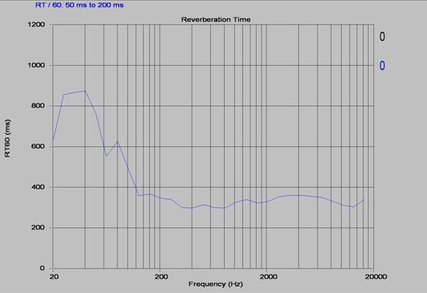
Lastly, let's take a look at our listening rooms. Listening rooms, have short reverberation times relative to our church, but long reverberation times relative to the control room mentioned above. Reverberation times for listening rooms vary depending on listener preferences including listening levels, and whether or not it is designed for multi-channel or 2 channel use. This is also an area where we can scientifically measure the reverberation times, but it's somewhat of an art to get the reverberation times correct for a particular listener-not unlike the differences in studios---what are the goals and what do we want to achieve. Some people feel that the listening room should not interact with the speakers, and it should perform much like the control room. Having listened in rooms designed like this, I can tell you I completely disagree. It takes away the kinetic energy of the music and having no interaction with the room has a very unnatural sound. In general we would like to achieve something between 0.34 and 0.39 seconds for an RT-60 from about 200 Hz on up. RT-60 measurements in small room acoustics below 200 Hz have little meaning and are flawed by the energy buildup of room modes. To evaluate bass response below 200 Hz, we have to use other methods.

Here is the reverberation time for an ideal 2 channel listening room:

Acoustical Measurements - Energy-Time Curves and Waterfall Plots

These can be very useful, although they can be more difficult to interpret as they are a steady state measurement at different times averaged for the entire frequency range, or a band of frequencies. So why would this be important? Well, like the reverberation times, we would like the energy at the frequencies to decay uniformly.

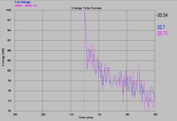
As stated above, one of the problems with energy time curves is that they can be difficult to interpret. Each curve is a very fast snap shot of what energy is present at that time. Because there may be comb filtering at that instance, it can sometimes be deceiving, but it's best to interpret the energy time curves by ignoring any dips in energy that rise again. The following graph shows energy time curves for the full range and the band from 4k to 8k. Notice that they track each other nicely. This is what is expected and is ideal:

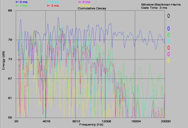
A subset of energy time curves is the cumulative decay plots. This is taken across the entire frequency range and is a snapshot at that particular time. The first is at 0 ms, and the subsequent snapshots can be at various intervals depending on what we are looking for. Ideally the 0 ms should be flat (it will have significant fluctuations due to comb filtering, but overall should be flat). If it's not flat, this generally means there is a problem with the equipment, because the direct wave response has no room interaction. This can be a great tool for troubleshooting. I was once sent a set of graphs that showed the cumulative decay at 0 ms (meaning the direct wave), where the frequency response was quite rolled off in the high end. The decay in the high end was not as rapid as everywhere else. The overall (meaning integrated for a long time) frequency response was pretty flat. I called the user and asked him if he had a treble control, he replied he did. I asked if it was turned all the way down-he responded yes. It turned out his room was very reflective with a lot of glass. The glass was leaking bass energy and reflecting the high frequency energy. He compensated for this "brightness", by turning the treble (tweeter in this case) all the way down.

Below is a different graph. One where the energy in the room is falling off rapidly at the high frequencies where the initial (0 ms) response was close to flat.

Waterfall Plots
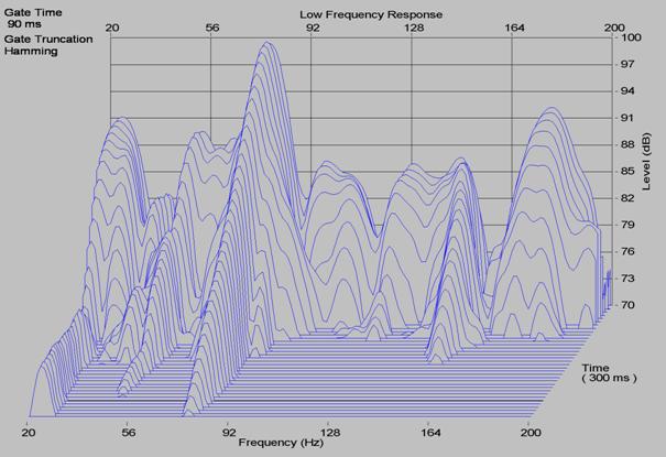
Eye candy? People have said this to me-waterfall plots are simply eye candy. I firmly disagree. Waterfall plots do look great, but they are very useful. In a simple 3-D snapshot we can see if everything is decaying uniformly. This is basically looking at the cumulative decay in different way. I like it because if I see one particular frequency that is being carried out much longer than all the others, I know it's a resonance of some sort-usually caused by the room. How long it's carried out has a lot to do with how significant that resonance is.

The graph below shows a prominent resonance frequency around 80 Hz:

Psycho-Acoustical Response Curve
This is a highly debated subject, and some might say controversial subject, but in our tests it has proven extremely useful. Some acousticians will say that the steady state response is all that you need and for trained acousticians, who may deal with this on a regular basis, this may well be the case. The basic premise of a psycho acoustical response curve is that it mimics in a 2-D graph what the human ear perceives relative to frequency response. Thus if there is a resonant mode it will be displayed as a peak at that frequency. The human ear has longer integration times at lower frequencies than at higher frequencies. Thus the gate time for the psycho-acoustical response curve is longer for low frequencies than high frequencies. Here is a psycho-acoustical response curve of the waterfall plot seen above.

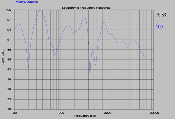
We use the psycho-acoustical response curve to set up the PARC. It is very easy to interpret and our results have worked out incredibly well by simply using the psycho-acoustical as our benchmark and bringing it's response as close to flat as is possible.

Special Note Regarding the Graphs
All measurements were taken using the Rives Audio Professional Test Kit. The analysis and display software is ETF from Acoustisoft. We have found this software and hardware to be the most cost effective method of obtaining state of the art measurements.

by Richard Rives Bird of Rives Audio

Resources and education in Acoustics: www.rivesaudio.com/educate

Contact Rives Audio: info@rivesaudio.com or 800-959-6553