Optimum Room Locations for Subwoofers An Analysis

Introduction

The placement of subwoofers and listeners in small rooms and the size and shape of the room all have profound influences on the resulting low frequency response.  For music playback in a small room, the overabundance or lack of bass energy is usually the most immediately noticeable audible characteristic, and varies greatly as you move about the room.  The use of multiple subwoofers at different locations in the room has been proposed in different ways to address the challenging issue of seat-to-seat variation.  Some subwoofer configurations are better than others.  Usually this depends on the room dimensions and seating layout.  What is optimal for one situation might not be optimal for another.

Room Simulation Motivation and Methods

My contribution to this problem has been to focus on rectangular rooms, using a simulation approach.  This allows me to look at large numbers of rooms instead of just a few, and compare them directly since the “room construction” is always identical.  It is a somewhat simplistic approach compared to the complexities of real rooms, so I don’t claim it to be 100% foolproof, just a useful guideline.  I have always focused first on reducing seat to seat variance in the subwoofer responses.  In a home theater or any other critical listening space, you don’t want one seat to have booming bass and another seat with weak bass.  Figure 1 shows an example of two acoustical measurements made at adjacent seats in a small room. Much larger differences could be expected for seats further apart. Modifying room acoustics and equalization won’t address this problem.  Using multiple subwoofers at the proper room locations can.

Figure 1.  Measurements at adjacent seats in a small room.

Using custom-developed room simulator software, the responses for a number of different subwoofer configurations and seating configurations have been predicted and documented in AES paper 8748 along with publicly available simulation results.  Each simulation was made not for just one room, but for a range of different room sizes.   In fact, over 30,000 rooms were simulated in all!  Before briefly describing the method and summarizing results, a couple of notes and caveats:

• This work is only relevant to rooms with multiple seats, since it is founded on the idea of reducing seat-to-seat variance. 

• This work only applies to rectangular rooms.   This simulation does not apply to a rectangular room with a large opening into another room.  A room where one wall is single layer sheetrock construction and the other walls are brick construction might be questionable due to very different acoustical properties of the walls at low frequencies. 

• Only “small” rooms are considered, up to 9 x 9 meters (30 x 30 feet). 

• Ceiling height is assumed to be 2.7 m (roughly 9 feet).  Results for 8 to 10 foot ceilings have been checked and found to not vary too much.

• Rooms are assumed to have low absorption, for two reasons: First, the equation used to predict subwoofer responses is only valid for the low absorption case.  Secondly, rooms where modes are an issue are most likely to be low absorption rooms anyway. 

• Finally, subwoofers are assumed to be bass-managed, i.e. all receiving the same signal low-passed from the pre-amp. 

Simulation Details

• Room size: L x W range is 4 x 4 m to 9 x 9 m, in 0.2 m steps. Ceiling height is 2.7 m.

• Acoustical absorption coefficient:  0.15 on all surfaces.

• Seating area: individual listener locations within the seating area “cloud” spaced at 0.2 m, randomized by up to 0.5 times the nominal spacing.  Height of seating area is 1.15 m +/- .45 m.

• Subwoofers locations at floor level, next to walls.

• Frequency range of interest: 20 to 80 Hz

The room simulator is based on the closed form solution of the wave equation in a rectangular room:

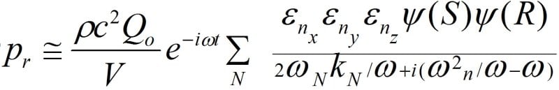
This equation gives the sound pressure  Pr for a given set of room dimensions and source (subwoofer) and listener location.  Since the exact seating positions aren’t known, seating areas are modeled using “clouds” of  “listeners” that generally fill in the seating area volume.  See an example in Figure 2.

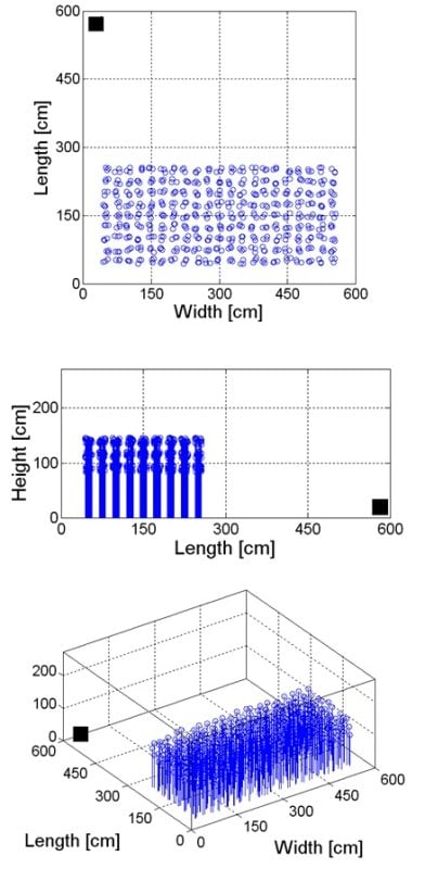
Figure 2.  Example of one particular set of room dimensions and one particular seating and subwoofer configuration.  Small stemmed circles are listener locations, while the filled rectangle is a subwoofer.  Plan, side and iso views shown for this 6 x 6 meter room.

Seven different subwoofer configurations and seven different seating configurations were simulated, giving a total of 49 different scenarios.  The subwoofer and seating configurations are shown in Figure 3. For each combination of subwoofer and seating configuration, rooms of various dimensions were simulated.  Specifically all possible room dimensions between 4 x 4 m and 9 x 9 m were simulated (in steps of 0.2 m).  This gives a total of 625 possible room sizes.  This gives over 30,000 individual rooms simulated, with up to 1000 listeners in each room.  The simulation software was implemented in Matlab, and optimized to run very fast!

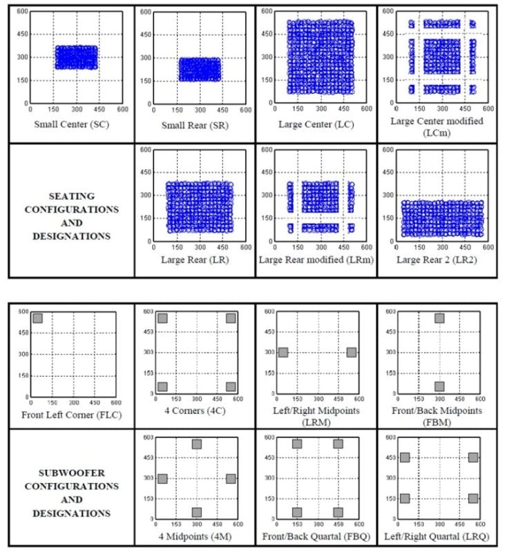
Figure 3. Seating and subwoofer configurations modeled. “Quartal” configurations are using positions on the wall which are at one quarter and three quarters of the length and width dimensions.

The output of the model is a magnitude response, from 20-80 Hz, at each listener location.  How can this be useful?  Some metric must be used to assign a figure of merit for each room simulation, so they can be plotted and compared.  The main metric used here is called “Mean Spatial Variance.”  It is a measure of seat to seat variation in the magnitude response (dB).  If you look at one frequency, you can calculate the variance of the magnitude response across all seats.  If you do this for each frequency, and average all the results, you get the MSV.  The smaller the MSV, the more similar the responses are from seat to seat (not necessarily flat, but similar).   Figure 4 shows a simplified example for two seats with low and high MSV values, and also illustrates again why it is important. Getting more consistent seat to seat responses makes equalization more effective.

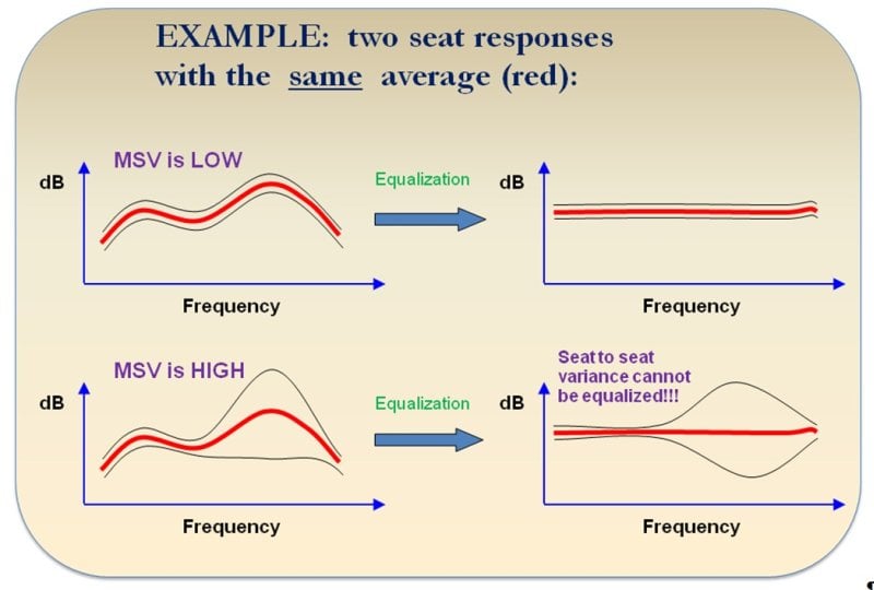
Figure 4.  Two simplified scenarios with different MSV values.

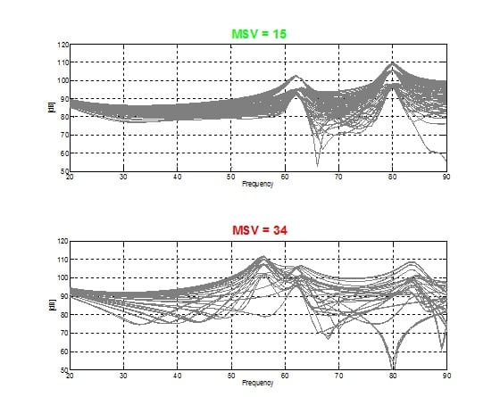
Figure 5.  Example of simulated frequency responses corresponding to a low MSV and a moderately high MSV.

We probably don’t want to ignore the total bass output in our quest for seat-to-seat consistency. Therefore let me introduce the Mean Output Level (MOL).  This is a very simple metric that gives a measure of how much low bass (20-40Hz) is generated on average in the seating area.  To calculate it, take the spatial average of magnitude response in dB over all listener locations in the model, then take the dB average of that curve from 20-40 Hz.  This gives a single number for MOL for a given room/subwoofer/seating configuration.  Note that we are averaging in dB, not sound power or sound pressure.  There is some controversy about which is most correct.  I will leave that for a separate discussion, and in any case I don’t believe it affects overall results too much one way or the other.   It makes sense to modify the MOL to account for the number of subwoofers.  Adding more subwoofers to a room, stacked in a corner for example, will make the MOL go up accordingly, but not due to any increase in efficiency.  To make the MOL metric relate more to efficiency, we subtract 10log(N) from it, where N is the number of subwoofers used.  This is referred to as MOLn, and is really a low frequency efficiency metric.

Results, Results, and more Results

So, we put all the room equation and room model information into a computer and crank the handle (at several gigahertz for a day or so) and out comes lots and lots of simulation data.  Now comes the interesting part.  Figure 6 shows a typical simulation result.

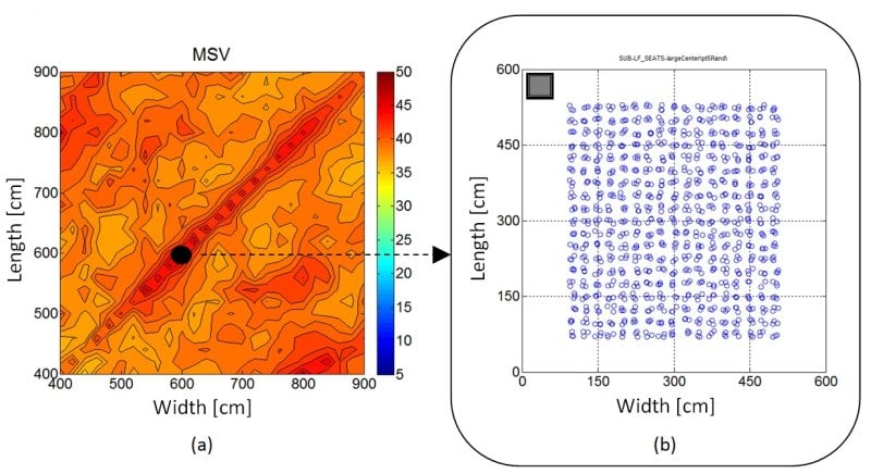
Figure 6.  Simulation results for a single sub in the front left corner and large centered seating area (a), and one particular set of room dimensions in (b).  Simulated metric is MSV.  Note that the figure in (b) is just one of the 625 room dimensions simulated, which are all represented at different points in (a).  Higher values of MSV (bad) show up as dark red in (a).

Figure 6 shows the Mean Spatial Variance (MSV) for all room sizes simulated, as a color plot.  The subwoofer configuration is Front Left Corner (“FLC”) and the seating configuration is Large Center (“LC”).  The right side shows a view of this configuration from the top, for the 6 x 6 meter dimension case.  Note that the listener locations that comprise the seating area “cloud” are randomized a bit for good measure.  The black dot on the left plot shows where this dimension set would be represented in the MSV plot.  Locations on this plot on the upper left triangle represent rooms that are longer than they are wide (the most typical case).  Locations on the lower right triangle represent rooms that are wider than they are long, and along the diagonal represents rooms with equal length and width.  Interesting to note in this plot is that these square rooms along the diagonal tend to have higher MSV values (i.e. darker red).  This means more seat-to-seat variance, and is undesirable.  SO, square rooms really are bad, like we have been told for decades…. Or are they?  We’ll get back to this.  The more inquisitive reader may wonder why the plot in figure 6 (a) is not perfectly symmetrical about the diagonal.  The answer is that it basically is; it is just that since the listener locations are randomized, the symmetry is thrown off slightly so that visually it doesn’t look perfectly symmetrical. Finally, note that in the simulation of different room dimensions, the seating area always scales proportionately with the room dimensions.

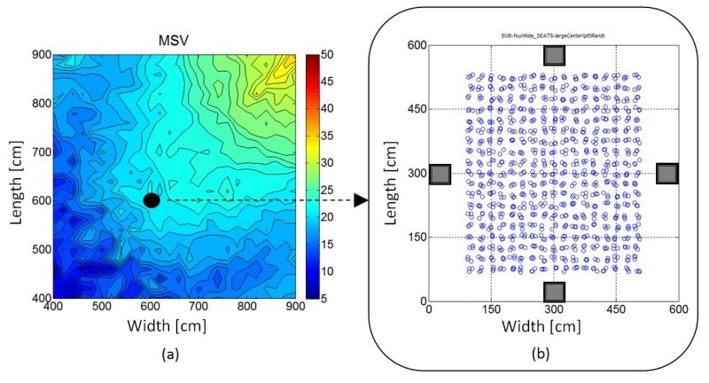
Figure 7.  Simulation result (a) for four subwoofers located at the wall midpoints and large centered seating area (b).  Simulated metric is MSV.

In Figure 7, we can see the effect of using four subwoofers and putting at the wall midpoints (“4M” seating configuration).  Note the general preponderance of blue to dark blue, representing significantly lower MSV values (good).  The range of 5 to 50 on the color plots for MSV really represents a full range of conditions from very consistent to wildly inconsistent seat-to-seat responses.  It is evident that the “4M” subwoofer configuration is much better than the “FLC” configuration in Figure 6 for all room sizes.  Another interesting observation is that the evidence for square rooms being bad, visible in figure 5, is not visible here!  So, square rooms are NOT necessarily bad as we have been told.  It depends on the subwoofer configuration.  So, we have a very useful observation already from the simulations.

What about Bass?

Why does the “4M” configuration give so much more seat-to-seat consistency?  The answer has to do with cancelling room modes.  A full discussion of this is not included here, but the effect on the low bass output (Mean Output Level normalized, MOLn) is of much interest.  After all, if we cancel modes, are we not losing some efficiency?  The answer is a qualified “yes”.  As might be expected, it will depend on the room configuration, and where the seating area is.  It is certainly possible to have reduced bass output overall in the room but happen to have higher bass energy where the seats are.  To continue with our example from Figures 6-7, Figure 8 shows MOLn results.  In the case of MOLn, higher numbers mean more bass, and are better.  For consistency, higher MOLn numbers are plotted as blue and lower MOLn number plotted as red.  So, as for the MSV plots, blue = good, red = bad.  In this case the MOLn numbers correlate to relative SPL values, as opposed to MSV which is a statistical descriptor.  In any case one can easily see that one sub in the corner gives much better bass efficiency for all room sizes than the four subs at wall midpoints.

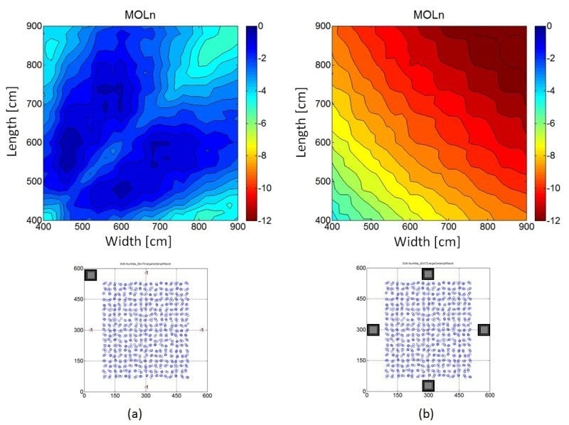
Figure 8. MOLn results from simulations, for Large Center (“LC”) seating configuration.  Subwoofer configurations are “FLC” (a) and “4M” (b).

So we gave up a lot of efficiency to get the seat-to-seat consistency.  However, this represents only two subwoofer configurations and one seating configuration.  There are many more possible.  Let’s look at another possibility.

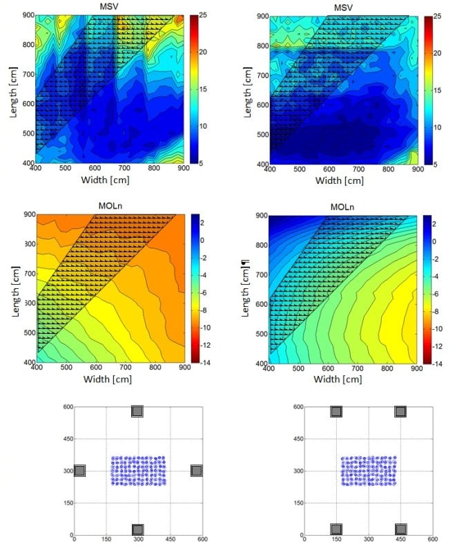
Figure 9.  Comparison of Four Midpoints (“4M”) to Front Back Quartal (“FBQ”) sub configurations for Small Center (“SC”) seating configuration.  Hatched area shows approximate room dimensions that would be more typical for a dedicated listening room. 

Figure 9 shows another seating configuration, called “Small Center” (“SC”) where the seating area is smaller and centered in the room.   Here we compare the 4 midpoint subwoofer configuration to another configuration where the subwoofers are located on the front and rear walls, one quarter of the total room width in from the side walls.  This is referred to as Front-Back Quartal (“FBQ”) configuration.  It can be seen that for this seating configuration the MSV results are equal to or better than the 4M configuration, while the MOLn is much improved.  SO, it is not always the case that you have to give up bass efficiency to get seat to seat consistency!

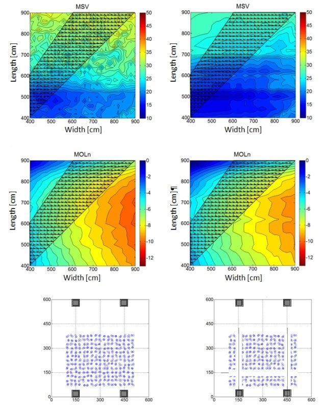
Figure 10.  Comparison of Front Back Quartal (“FBQ”) sub configuration and Large Rear (“LR”) seating configuration, and with seats along the ¼ room dimension lines removed.  Hatched area shows approximate room dimensions, which would be more typical for a dedicated listening room.

Finally, in Figure 10 we can see the effect of removing seats along the room dimension quartal lines.  Past investigations have suggested that this is an area where modal effects may be more prominent.  Sure enough, removing these seats caused a marked improvement in the MSV metric.  The effect on MOLn was very small.

Many other interesting observations can be made from looking at the simulations.  For example, the “4M” subwoofer configuration seems to be fairly insensitive to room dimensions and produces results that are more closely related to room volume.  See figure 11 for an example.   In such a case, calculations of required subwoofer output capability for a given room would be simplified.

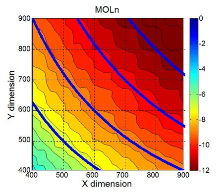
Figure 11. MOLn results for “LC” seating configuration and “4M” subwoofer configuration.  Lines of constant room volume are also shown (heavy blue lines).

Averaged Results

The following tables show results of the simulations when data for the entire range of room dimensions are averaged.  Hopefully, the attentive reader will remember that this is only of interest in the most general sense.  Any time actual room dimensions are known, this table is not representative and should not be used.  Go to the simulation library and look up your room!

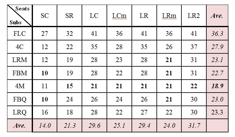
Table 1. Mean MSV values for different subwoofer and seating configurations averaged for all room dimensions.  LOWER values equate to better performance for this metric.  Best values for each seating configuration are in bold type.  Averaged values for each column and row are also shown.

Table 1 shows MSV values, averaged for all room dimensions.  Bolded values are the best for each seating configuration.  Best overall is the 4M subwoofer configuration.  Worst is the sub in one corner (FLC).  Subs in four corners (4C) is second worst.

Table 2. Mean MOL values for different subwoofer and seating configurations averaged for all room dimensions.  HIGHER values equate to better performance for this metric.  Best values for each seating configuration are in bold type.  Averaged values for each column and row are also shown.

Table 2 shows MOL values.  Best overall is sub in one corner (FLC).  Worst are the 2 subs at opposing wall midpoints (LRM and FBM).  Subs in four corners (4C) does very well, nearly as good as the FLC.

Comparing Tables 1 and 2, the “Quartal” configurations (FBQ and LRQ) are good compromises for MSV and MOL, i.e. they provide good seat to seat consistency and good low frequency support (again ignoring specific room dimensions for the moment).

Conclusions

So far, we have barely scratched the surface of what can be gleaned from the simulation results.  Some additional observations are included in the AES paper.   From the examples shown here and from reviewing the full simulation “library” it is apparent that there is a large effect  from changing seating /subwoofer configurations and room dimensions, and that this can used used to great advantage!  This is much more powerful than just using very general rules of thumb (like “just throw the subs in the corners”).  The biggest single takeaway from all of this is that rules of thumb about which subwoofer configurations work best are of limited use if you don’t take seating configuration and room dimensions into account. SO, how can this be done?  How can these simulation results be of practical use?  If you are designing a room and have some latitude as to dimensions, seating and subwoofer configurations, you should be able to look at the data and find a combination which best fits your goals gives the best possible results.  If one or two of these variables are fixed, you can make the best selection for the remaining one(s).  If all three of these variables are fixed, the only thing left would be some optimization of the level, delay and filtering for the subwoofers – a subject for another day.

Terms

• Listener Locations: Individual locations where the room response is calculated in the room model.  A “cloud” of these represents a seating area.
• Subwoofer Configuration: Refers only to the number and locations of subs in a room.
• Seating Configuration: Refers to the general area within which seats are located in a room.
• Mean Spatial Variance (MSV): A metric describing how much variation there is in the magnitude response (in dB) between listener locations in a given seating area.  It says nothing about flatness of response, only seat to seat variation.  Units are dB2.  Larger numbers mean more variance, less consistent.
• Mean Output Level normalized (MOLn): A metric for quantifying the relative efficiency of the subwoofer configuration at low frequencies (20-40 Hz).  It is derived from the averaged response in the seating area.  The total number of subs is accounted for so that a configuration with more subwoofers does not automatically give a higher MOLn value.  It is thus an efficiency metric.

Acknowledgements:

Todd  would like to thank Dr. Floyd Toole for winding him up and pointing him in the right direction on this very topic.  Audioholics is thankful to Todd and Harman for taking the time to share insights on subwoofer placement with us.