
NHT Xd Loudspeaker System Review
- Product Name: NHT Xd Loudspeaker System
- Manufacturer: NHT
- Performance Rating:

- Value Rating:
- Review Date: May 04, 2007 18:09
- MSRP: $ 6000
|
Model Name/Number: |
NHT XdA Power Amp/DSP Processor |
|
Model Name/Number:
|
XdS Loudspeaker 2.1 kHz |
|
Model Name/Number: |
XdW Bass Module |
Pros
- Near-holographic imaging & soundstaging
- Peerless tonal neutrality
- Firmware upgradeable, provisions for future room setup capabilities
Cons
- No component mix-n-match
- Expensive
- Limited finish options
Introduction
Life is good as an audioholic writing reviews for Audioholics. And one of the nicest things about being in this fortunate circumstance is Gene never sends junk. Ever. (I’ve asked him on occasion to send some suitable specimens of junk, ripe for public skewering, but he’s never been inclined to do so). So in my brief time as a reviewer for Audioholics I’ve been in a fortunate position to find a stream of quality products being delivered to my front door. A fine case in point, and the topic of this review’s conversation, is the NHT Xd system. If I had to describe the system in one sentence I would say, without reservation, here is a system that actually lives up to all the hype. And looks pretty cool doing it, too
Since its incorporation in December of 1986, NHT has, by anyone’s measure, lead a storied existence:
definitely a company that has seen its share of ups and downs. (For those interested, the 5/91 edition of SpeakerBuilder magazine features Bruce Edgar interviewing Ken Kantor, an NHT co-founder, discussing the challenges of sheparding a startup along with an insiders technical guide to the engineering that had gone into there earlier products, such as the Model 1 & 2).
Through it all, NHT have managed to bring to market consistently innovative products, notably forward thinking in design. The Xd system is just such a product. A hybrid, if you will, of advanced speaker, amplifier and digital processing technology that all adds up to one sweet listening experience, sure to surprise & satisfy demanding audio palates everywhere.
First Impressions
So what exactly do you get for $6000.00 US (MSRP)?
In a nutshell, you get a pair of XdS each sporting a 1” tweeter & 5.25” midrange driver, (with stands & cabling) the XdW (a bass module) packing 2 10” woofers and its own built-in PowerPhysics 500 W Class D power amp & cabling, and the XdA, a Deqx/PowerPhysics processor/power amp with 6 channels of DSP processing, 4 x 150 W amplification channels, 2 line level outs, firmware upgradeable via USB. Though tempting at first glance to think so, its definitely not a satellite/subwoofer system, typical or otherwise.

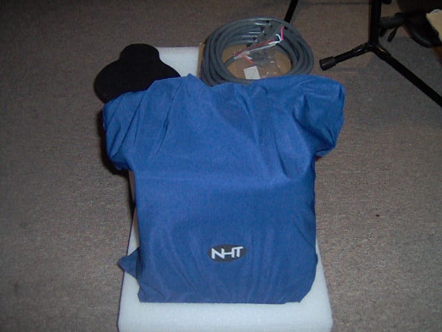
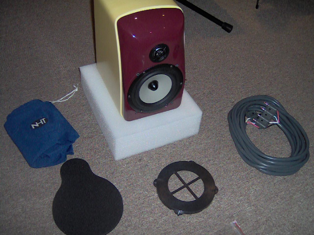
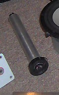
Figures 1 – 3: Unpacking an XdS. Note the cover for the woofer, used during shipment for protective purposes. Note also the 4-pin banana plug found at the end of the coiled speaker cable, also in Fig. 3 and parked just to the right of the woofer’s protective cover. The big blue sock keeps the Xd’s superb finish in pristine condition.
“Retro moderne” is how an interior designer friend of mine described the appearance of the system.
The burgundy/cream color combination of the supplied review system is a classic and the overall look is reminiscent of the Raymond Loewy school of industrial design. “Entirely new, yet entirely familiar” is another phrase she used to describe the visual impact of the system. The Xd system is a unique looking product, that doesn’t take an advanced degree in the visual arts to appreciate. The folks at NHT must have thought long and hard where it came to crafting the appearance of the system. It has a way of growing on you and though the system has graced my listening room for a considerable length of time, the novelty hasn’t worn off, either. It’s as cool looking today as the day is was first unpacked.
NHT XdS Build Quality & Design Overview
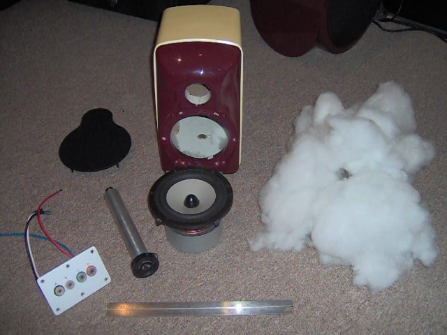
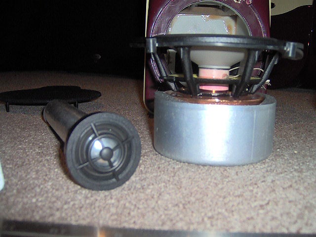
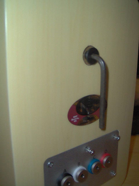
Figures 4 – 7. 4: XdS Unplugged: Cabinet,
stuffing & grill cloth, drivers. (Note
absence of any crossover coonected to the input jacks seen at lower left of
picture), 12” ruler for scale; 5: XdS
drivers; 6: Tweeter/heat sink close up (note metal tube attached to tweeter
back); and 7: Cabinet backpanel. Allen wrench hanging from bolt that holds the
distal end of the tweeter’s heatsink in place. Note color-coded jack panel at
bottom of photo.
XdS Midrange Driver
Rather than simply
packing the Xd system with cheap drivers and letting the XdA’s DSP functions pick
up the slack, NHT have opted for fitting out the system with a collection of
premium-grade drivers.
The XdS midrange
driver is a 5.25” magnesium alloy, tapered cone unit sourced from SEAS, a
Norwegian high-end manufacturer. The frame is cast aluminum/magnesium alloy. It
features a rubber roll surround, exposed pole pieces and magnetic shielding. Sound
reflection, air flow noise & cavity resonance are all minimized by the
comparatively large basket frame openings.
It has a free air resonance, fs ≈ 48 Hz. Visually speaking, it
bears a family resemblance to the SEAS Excel W15CY001, a drive unit not unknown
in DIY circles.
XdS Tweeter
The XdS tweeter (also
sourced from SEAS) features a 26mm aluminum/magnesium dome, self-shielding neodymium
motor structure, underhung voice coil, a magnetic fluid-filled gap and a
comparatively wide roll surround. (With both drivers magnetically shielded, the
XdS is a CRT display-friendly system). The tweeters free air resonance sits at
about 1.6 kHz and its first break mode can be found at about 26 kHz.
XdS Cabinet
The XdS cabinet is a classic study in industrial art, rich
in the features of an aesthetically successful merging of form & function.
Here, basic design principles – driver offset, rounded faceplate edges, relatively
inert, crossbraced cabinet panels and so forth - are all sculpted into a
visually attractive presentation that has a way of positively growing on you
the more you look at it. You won’t go hunting for an unobtrusive spot in your
listening space’s terrain to hide them away. On the contrary: you’ll likely
catch yourself looking for spots that highlight
these latest additions to your art collection. They’d look right at home in the
Guggenheim museum (5th
Avenue between 88th & 89th
Streets in Manhattan).
The XdS cabinet is a comparatively small (10.25”H x 6.5”W x
8.5”D), totally enclosed (acoustic suspension) construct comprising panels of
MDF and a faceplate made of a dense composite material referred to as “BMC”. Internally,
it is cross-braced and heavily stuffed. The stands supplied with each XdS are,
visually speaking, perfectly complementary, weighted for maximum stability and
put the XdS at an ideal height for seated listening. The stands are made from pure MDF, except the
base which has a ¼” thick steel plate in it for stability. They weigh in at
18.5 lbs. Clamps, thoughtfully located down the back of the each stand’s spine,
help keep the system’s cabling neat and out of sight. Great idea and typical of
the attention that has obviously been paid to the details of the system. Spikes
are a provided option.
XdS Crossover
There isn’t one. At least not the usual
inductor/capacitor/resistor passive crossover commonlyfound inside a more typical loudspeaker. In actuality, all
crossover functions are handled upstream by the XdA DSP. (More about this momentarily). One
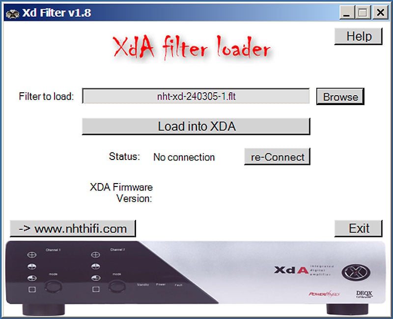
particularly interesting feature that, to a degree, obsolescent-proofs the XdS is
that the filter functions are implemented as firmware that’s updateable/changeable
via the XdA’s USB port, all handled via a loader utility you install on your PC
or laptop. Various filters along with other useful downloads are available at
the NHT website.
XdW
Bass Module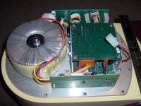

The XdW is a
powered, acoustic suspension, LF system featuring two opposing 10” CNC-machined
aluminum cone drivers, a 500W Class D amp and a notably sparse control panel
bolted into the back of the unit. There you’ll find an on/off switch, trim (“Less”
“Just Right” and “More, i.e., -10 dB, 0 dB, +10 dB), voltage selector and
balanced input jack. Like the XdS, all processing occurs upstream, in the XdA’s
DSP. On carpet, its surprisingly easy to maneuver around while, for example,
you’re looking for the sonically ideal place for it in your listening room.
Remove the control panel and you’re looking at the power amp, seen at right. You’ll also see the space formerly occupied by the amp is sectioned off from the rest of the cabinet’s internal volume by a bulkhead through which the leads connecting the amp with the drivers are routed. The bulkhead prevents, in a simple, straightforward fashion, any wind noise emanating from openings in the control panel when the sub is active – a not an uncommon problem seen elsewhere.
The approach NHT have taken in using the opposing drivers effectively minimizes cabinet panel vibration. So, even though the XdW can be easily maneuvered around your listening space’s carpeting come set up time, it won’t vibrate itself around the floor or impart much mechanically-induced noise to neighboring rooms. A real boon to apartment dwellers or to those otherwise surrounded by noise-sensitive neighbors.
Fit & finish were superb all the way around. In terms of the finish, not a flaw or blemish were apparent anywhere – anywhere - on either XdS, their respective stands or the XdW. Even after going over each with a chamois cloth was there anything found that looked out of place. Outstanding! Construction was of an equally high caliber. These cabinets, the stands – all of it - are solid. The faceplate of the XdS – made of a composite material and molded into a smooth, flowing construct – is a particularly good example of the abundance of quality apparent in the architecture that is this system. I really wouldn’t be too terribly surprised if an Xd system ended up on display in a museum of modern art somewhere. Would that more of the things we surround ourselves with looked this good!
XdA Processor/Power Amp
The XdA is a hybrid of advanced technologies, melded into a product with a decidedly uncluttered, yet high-tech appearance. That self-same outward simplicity grandly belies the complexity that lurks just beneath the cover.
On the back panel you’ll find the On/Off switch, speaker-level outputs for both XdS, trigger jack with mode switch (In, Ext, Audio), analog (balanced & unbalanced) stereo pair inputs, balanced microphone input & one pair of balanced & unbalanced line-level outputs for use with up to 2 XdWs. The front features mode (boundary compensation filter preset) control buttons, their attendant indicator lights and nothing else.
The XdA’s brawn resides with 4 individual 150W Class D power amps. They’re designed and built by PowerPhysics, a relative newcomer to the audio scene, based in Newport Beach, California. The XdA’s amps sport an eye-popping efficiency factor of ~ 95%, which simply means more of the electrical energy fed in to the XdA gets fed out to the XdS speakers; less gets wasted as heat. (Compare the XdA’s ~95% amplifier efficiency with the ~20%, of a typical Class A or the ~50% Class AB linear amplifiers). Running at such a high rate of efficiency also means the various semiconductor’s junction temperatures are kept comparatively low which in turn means the XdA does not require any heavy, complex or costly cooling hardware to deliver the (electrical) goods.
Figure 8: Simplified Circuit Diagram, Class D power amp.
At the heart of the extraordinary efficiency performance demonstrated by D class power amps such as those found in the XdA, is the use of semiconductors as switches, seen at upper left in the circuit diagram showing above. When “On” high current at a comparatively low voltage flows, hence little energy is lost. When the switch is “off”, there’s no current flow and no energy loss. Essentially, the incoming audio signal is used to modulate the PWM carrier that drives the output devices.
The resulting (now amplified) signal is then fed through a lowpass filter stage (seen at upper right) to remove the PWM carrier component of the output. PowerPhysics has taken this semiconductor–as-switch design approach one step further and have been awarded a patent (US, #6084450) for their efforts. At risk of oversimplification, PowerPhysics have devised an elegant non-linear control method that further increases (!) efficiency, lowers power source regulation requirements and forces errors between the reference & switching variable to zero at each cycle.
The XdA’s considerable processing power resides, of course, in its DSP processor sections. Designed by DEQX (Brookvale, Australia), it presents with quite a substantial collection of noteworthy specs. The XdA’s processor section controls everything the 6 output sections (4 for the Xds’ and 2 for up to two XdWs) from crossover frequency point & resolution, crossover type & order (capable of up to 300 dB/octave!), amplitude, phase, & group delay correction to time alignment and so forth. The DSP board in the XdA was done by DEQX and NHT. The amplifiers and power supply were done by Power Physics. All other aspects of the XdA were designed by NHT And the firmware at its core is entirely updateable. In short, the DEQX DSP controls the performance envelope of the system to an all-encompassing degree and with a flexibility that isn’t found in more ordinary speakers. In addition, NHT are planning for the XdA’s future a mic-based end-user system setup/calibration feature. The necessary mic jack is already in place on the XdA’s back panel. A pre-amp/AVR is needed to drive the XdA as it does not provide for source selection, level adjustment and so forth; all preamp functions have been kept out of the processor.
NHT XdS Setup
 Fun begins
with the arrival of 6 sturdy, well packed cartons, each containing an
individually wrapped system component. (See Figs. 1 – 3, unpacking one of the
XdS). After liberating the individual works of art that make up the Xd system,
you’ll have arrayed before you a pair of XdS speakers, the XdA power
amp/processor, the XdW powered woofer, stands for the XdS, along with all
required cableage (a pair of 25’ speaker cables & a 25’ line level XLR –
XLR cable to connect the XdA to the XdW), power cords, spikes, rubber pads,
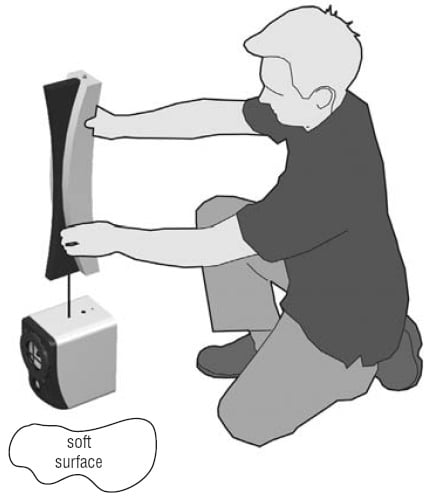
manual and some smaller accessories. The
minimal assembly required was straightforward and built of a series of simple
steps, all more than adequately illustrated in the manual. As an example, the
section of the manual illustrating joining the stand to an XdS is given at
right.
Fun begins
with the arrival of 6 sturdy, well packed cartons, each containing an
individually wrapped system component. (See Figs. 1 – 3, unpacking one of the
XdS). After liberating the individual works of art that make up the Xd system,
you’ll have arrayed before you a pair of XdS speakers, the XdA power
amp/processor, the XdW powered woofer, stands for the XdS, along with all
required cableage (a pair of 25’ speaker cables & a 25’ line level XLR –
XLR cable to connect the XdA to the XdW), power cords, spikes, rubber pads,
manual and some smaller accessories. The
minimal assembly required was straightforward and built of a series of simple
steps, all more than adequately illustrated in the manual. As an example, the
section of the manual illustrating joining the stand to an XdS is given at
right.
Keep the manual handy during assembly. Speaking of which,
prior to assembly and using the system I highly
recommend reading the manual. It’s an easy & informative read: it’ll only
take a few minutes and well worth the small investment in time. All told, it
took about 15 minutes or so to get the system unpacked, assembled, positioned and
ready to go. I used an AVR’s front right & left pre-amp outs to drive the
XdA. All in all, the Xd system is about as plug and play as it gets. It took no
more effort than that required to assemble & place a couple of floor lamps.
NHT have obviously put a great deal of thought into making the assembly and usage of the Xd system as simple & easy as possible. One downside (if there is such a thing in this case) to this otherwise positive circumstance is that something so easy is easily rushed. When I first unpacked the Xd system, I quickly read through the manual, familiarized myself with the assembly procedures, put the system together, moved it into place and began the recreational listening portion of the system assessment - and the system kept switching itself off! On particularly quiet material this would happen so often I wouldn’t even bother listening all the way to the end of the CD. What was wrong with this thing? Actually, nothing whatsoever.
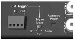 The XdA ships
with its external trigger set to switch the amp on or off (“Audio”) depending
on whether or not it senses an incoming audio signal. In my hasty read through
of the manual, I had not paid attention to this essential fact. Had I done so,
I would have switched the trigger to “On” mode, as in always on when the XdA is
on, (and where it has been set since) and spared myself any unnecessary grief. Read
the manual!
The XdA ships
with its external trigger set to switch the amp on or off (“Audio”) depending
on whether or not it senses an incoming audio signal. In my hasty read through
of the manual, I had not paid attention to this essential fact. Had I done so,
I would have switched the trigger to “On” mode, as in always on when the XdA is
on, (and where it has been set since) and spared myself any unnecessary grief. Read
the manual!
Placement was easy. The general location for the 2 XdS had been predetermined by having an accomplice walk the room while reading from a book. Changes in the tonal balance of the voice helped to narrow the field of suitable candidate positions. In the end, they were located at just over a meter in front of the back wall and slightly less distant from each of their respective side walls. The XdW was located between them and approximately .3 meter behind the plane formed by the XdS faceplates. Though the XdA can easily drive 2 XdW bass modules, only one unit was supplied for this review. The XdA was parked beside the AVR driving it, easy to do given the generous cable lengths supplied with the system.
NHT XdS Listening Tests
Auditioning the Xd system is a purely pleasurable exercise
in musical exploration. There are so many sonically compelling musical
strengths inherent to the Xd its hard to tear yourself away from the system
when life’s other commitments require your presence elsewhere. It’s also hard
to know where to start in describing these many, many strengths; if you’ve had
the opportunity to listen to an XdS system, you’ll likely know there are so
many competing for your immediate attention. Ah, such are these sweet
challenges. Onward to the subjective assessment.
 First up on deck is the Yellowjackets’ “time squared” CD,
(HUCD 3075). The Yellowjackets have been around for what by now seems like
ages. They’ve always had a sound (jazz fusionists with pronounced old school
sensibilities) that seems especially well showcased by systems possessing
unusually low mechanical/acoustical noise floors. (Read: musical details don’t
get lost beneath the grunge). Sonically speaking, a system with as low a noise floor
as the Xd is analogous to a video projector with a contrast ratio in the 5 or 6
figures – consciously or not it’ll become a standard by which all others are
judged.
First up on deck is the Yellowjackets’ “time squared” CD,
(HUCD 3075). The Yellowjackets have been around for what by now seems like
ages. They’ve always had a sound (jazz fusionists with pronounced old school
sensibilities) that seems especially well showcased by systems possessing
unusually low mechanical/acoustical noise floors. (Read: musical details don’t
get lost beneath the grunge). Sonically speaking, a system with as low a noise floor
as the Xd is analogous to a video projector with a contrast ratio in the 5 or 6
figures – consciously or not it’ll become a standard by which all others are
judged.
Track after track, the Xd system filled the listening space
with a sound stage that was as high as it was wide. Imaging bordered on the
holographic (due in part to the Xd’s tightly controlled impulse response and
immaculate tonal balance), with the various instruments definitively painted
across the sound stage, each clearly defined in their location. The XdS did all
this while at the same time presenting a rather convincing illusion that they
had nothing to do with the music you were hearing; they were invisible; the
music was simply there in the space before you.
Tonally speaking the Xd system at times resembled that of some
of the best electrostatic systems out there, with the added punch of the XdW
thrown into the bargain. With as expansive and sonically clean a sound stage as
that presented by the Xd system, it was easy to get a sense of the space around
the various instruments, further adding to the illusion of being right there.
The Yellowjackets compositions will typically make lively
use of whatever dynamic range any particular playback system can provide. Biamped and
powered by a total of four separate 150W rms (300W, peak) Amplifiers, plus the XdW’s own 500W rms (700W, peak) power
amp the Xd system was able to provide a dynamic range easily capable of supporting the demands of
the playback material, delivered at realistic levels at the listening position.
For example, the sax in “Monks Habit” or “Claire @ 18” was presented at a level
I would expect if it were the band and not the speakers situated 10 feet in
front of the listening position. The bass lines never disappeared, always
clean, always focused. The drum/ percussion tracks were arrayed across the
sound stage so stably the individual instruments never seemed to waver in their
relative position, further enhancing the illusion of 3-dimensional acoustical
reality. Off-axis performance was, given the systems multitude of well-executed
design attributes, outstanding as well.
Next up on deck was the sampler CD included with the Xd
system, titled, appropriately enough, the NHT Xd Sampler, The E.S.E Sessions. The sampler sports 5
tracks of superbly recorded, mixed and mastered material - vocals and
unamplified strings (dobros, slide guitar, bass, nylon-stringed guitar) -and nothing else.
Perfect for a mellow or nearly meditative listening experience. Long before the CD came to an end I’d made a
mental note to look up Blue Coast Records and add more of their fine product to my CD collection.
This CD, right from the first track, “Looking for A Home”
takes the Xd system right to the edge of its musical envelope, involving you in the essence of the
individual performances, never dropping the ball where it comes to the subtle
details that separate music produced from music reproduced. The harmonic
structure of the voices and the delicate interplay of the instruments were
portrayed in a way that leaves one wishing everything in your CD collection
could sound this good.
In the second track “Slow Day” the XdW bass module gets a
work out. In this particular track the melodic acoustic bass line weaves a masterfully
crafted underpinning that shows off just how musically accurate, the XdW, under
the wizened digital guidance of the XdA really, really is. In this case, the
bass line is an equal partner with the vocals and guitar, never intruding but
always supporting the melody. (Think of the bass line in Zeppelin’s “Ramble On”
and you’ve got the idea). In thinking
about it afterwards, I realized I’d been so impressed with the job the XdW bass
module had done in convincing me the illusion was real that all the while I’d
been listening to the track I’d been speculating as to how they’d managed to
capture such a true-to-life rendition of the acoustic bass (far harder to do
than it sounds). Another words, my focus
had been drawn into the session and I had forgotten about the speakers, they’d
done such a good job of disappearing, convincing the ear they had nothing to do
with the music being heard. Excellent!
Track 4 “Darcy Farrow” showed off the systems ability to subjectively
reach for and grab the sharp transients presented by the Dobro (thanks in equal
measure to the tweeter’s design and the electronics driving it) while
maintaining beautifully the harmonic structure of the slide guitar. (A
testament to not only the quality of the individual components but also how
well they integrate). With power to spare the system was well able to
accurately convey the dynamic range of the performance, all at realistic levels. With loud, musically
complex recordings, masking can hide all sorts of failings. With more (so to
speak) sparse recordings - like an acoustic guitar & a lone Dobro – any
such failings will stand out. That, of
course, includes the speakers. One example that immediately comes to mind is
the case where the midrange driver & the tweeter don’t integrate well;
Dobros end up sounding like they’re made of plastic (they definitely aren’t)! The
Xd system had no such problems.
On other material (various recordings of Gershwin’s Rhapsody In Blue and the first couple of
Van Halen albums) I did bump in to the system’s limits. And all systems – regardless
of the size of the price tag or the amount of competent engineering that went into their
creation – certainly have limits.
I’d read elsewhere that others had encountered a bit of
noisiness with the system. Everything from purported ground-loop hum to
processor “hiss”. I found it did indeed
hiss a bit, but in the case of the system provided for this review you’d have
to be impractically close to either XdS to actually hear the hiss. If you’re in
the habit of wearing your speakers like headphones (many years ago I saw
someone try this at a frat party once), then, sure, you’ll hear it. Otherwise,
even when playing back solo piano material like Gershwin’s Rhapsody In Blue it wasn’t audible at the listening position. As
well, I had no problems whatsoever with ground loop hum, even though the system
had been connected in a way that theoretically could have set it up for just
such problems.
I’ve also seen questions arise elsewhere considering the
system’s power-handling ability or perhaps more to the point how loud it can
play.
 I found that extreme levels (early Van Halen albums,
cranked) you could hear the midranges struggling a bit in their lower registers, but this occurred at
playback levels that were extreme and used only once to see just what the
limits were. Under all other operating conditions tested, the system functioned
flawlessly. Its not all that difficult to imagine just how loud the system can
play when you stop to consider you have a pair of tweeters, each powered by its
own 150W rms amplifier, a pair of midranges, each powered by its own 150W rms
power amp and a bass module sporting a pair of 10” drivers, fed by its own 500W
amp. Of course, if you need a bit more, you can add a second XdW and upgrade
the firmware.
I found that extreme levels (early Van Halen albums,
cranked) you could hear the midranges struggling a bit in their lower registers, but this occurred at
playback levels that were extreme and used only once to see just what the
limits were. Under all other operating conditions tested, the system functioned
flawlessly. Its not all that difficult to imagine just how loud the system can
play when you stop to consider you have a pair of tweeters, each powered by its
own 150W rms amplifier, a pair of midranges, each powered by its own 150W rms
power amp and a bass module sporting a pair of 10” drivers, fed by its own 500W
amp. Of course, if you need a bit more, you can add a second XdW and upgrade
the firmware.
NHS XdS Measurements and Analysis
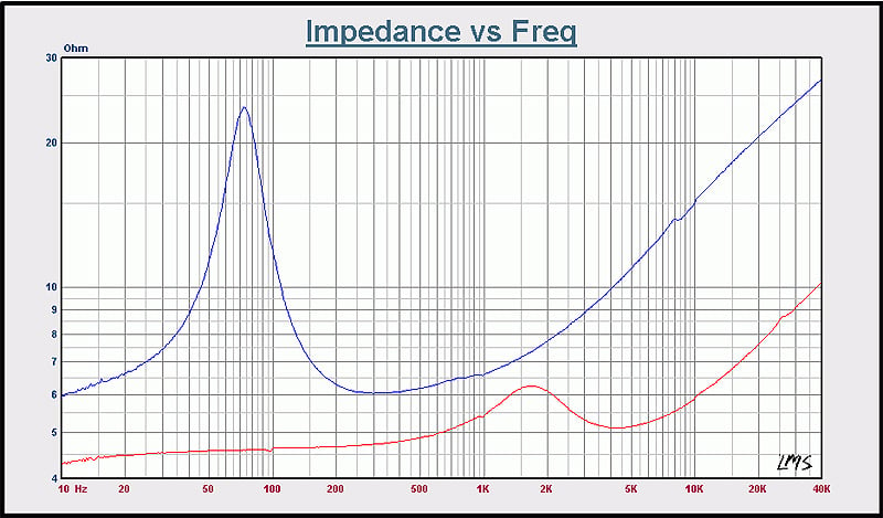
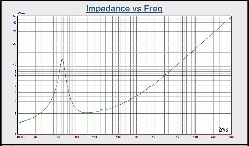
Figure 1a & b: Impedance & Phase. At Left: XdS midrange (blue) and tweeter (red). At right: XdW
A series of measurements were undertaken to develop an objective assessment of the Xd system.
In figure 1a & b we see the impedance scans derived from measuring the various drivers. These measurements were done with the drivers in their respective cabinets. At left are the midrange (blue) and tweeter (red) impedance curves for one of the XdS. Both are clear of any of the sort of anomalies that would arise owing to mechanical resonances and so forth. The design of the cabinet, the mechanical properties of the materials used in its construction, as well as the substantial amount of stuffing packed into the cabinet’s internal volume all contribute to this particularly clean looking plot. (As a side note, the slight glitches that show, for example, at 100 Hz, 1kHz, and 10kHz on the tweeters impedance curve are measurement artifacts generated by the LMS card that was used in capturing the data and are not symptoms of any sort of underlying driver/system pathology). The blue curve seen at left is typical for a totally enclosed cabinet, with its single Z-peak seen at left. The peak itself, appearing as it does at about 72 Hz, indicates the system is tuned lower than the high-pass knee of XdS’ intended acoustical response, thus helping to keep cone excursion within well controlled limits The tweeter’s curve (red) indicates an in-cabinet resonance frequency of about 1.6 kHz and the general appearance of the curves that lie just to the left & right of the peak are typical for fluid-cooled tweeters, such as those used in the XdS. Like its midrange counterpart, it too sports an in-cabinet Z-peak lower than the high-pass knee of its intended acoustical response, once again helping to keep cone excursion within well controlled limits, in turn helping keep distortion down as well. At the upper end of the tweeter’s z-curve, in the 27 – 28 kHz region, are a few barely discernible glitches indicating the tweeter’s metal cone entering its primary breakup mode.
The green curve seen at right is the impedance curve for the XdW. For this measurement, the built in power amp was removed from the XdW, exposing the leads connected to the two 10” drivers. As before, impedance data were taken with the drivers in place and in the cabinet. The curve presented here, like that showing for the XdS’ midrange driver, is typical for that of a system featuring a totally enclosed box. The location of the peak indicates the system is tuned to about 55 Hz. The only noticeable glitch is seen at ~ 250 Hz. Whatever the underlying cause, there was no parallel anomaly seen in the amplitude response plot of the XdW.
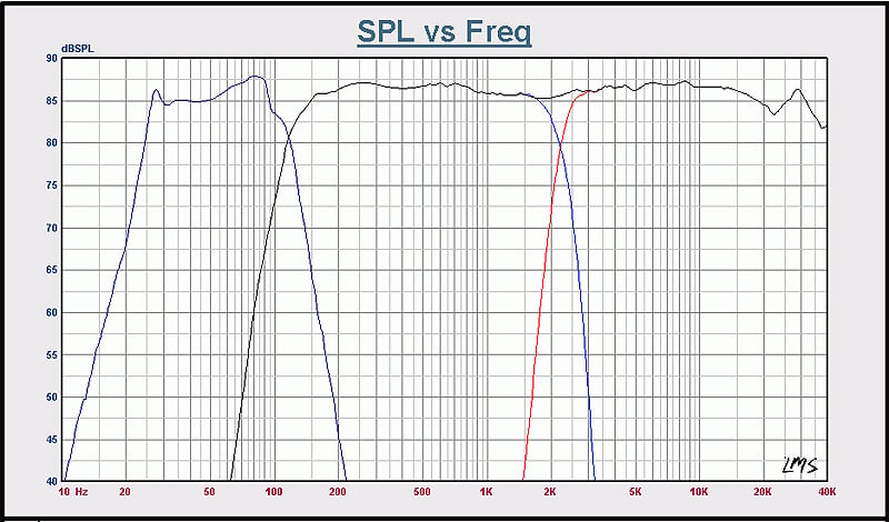
Figure 2: System response, dB spl. Dark blue: XdW; Black: XdS combined tweeter (red) & Midrange (blue) Response. 1/12th Octave smoothing employed for improved visual clarity
In figure 2 the system amplitude response plot curves, in dB spl, are shown for the XdS tweeter (red), midrange driver (blue), their combined response (black) and that of the XdW (dark blue). A variety of measurement approaches were employed and the results were scaled to 1m. The XdA was driven by the LMS card at a voltage just above that needed to produce amplitude response plots consistent with the sensitivity of the system, as determined by deriving the midrange driver’s Thiele/Small parameters. Another words, the plots are a dB or two above actual system sensitivity.
Of particular note here are the remarkably steep (acoustic) crossover slopes seen in Figure 2 as well as the tweeter’s response affected by the metal dome entering its first breakup mode above 20 kHz. The general appearance of the system’s amplitude response in the ~ 1 kHz to 10 kHz range illustrates the electrostatic-like subjective impression mentioned earlier, made by the XdS system. The XdW bass module supplied for this review has useful response down to around 25 Hz and consistently surprised and impressed with the quality of its performance.
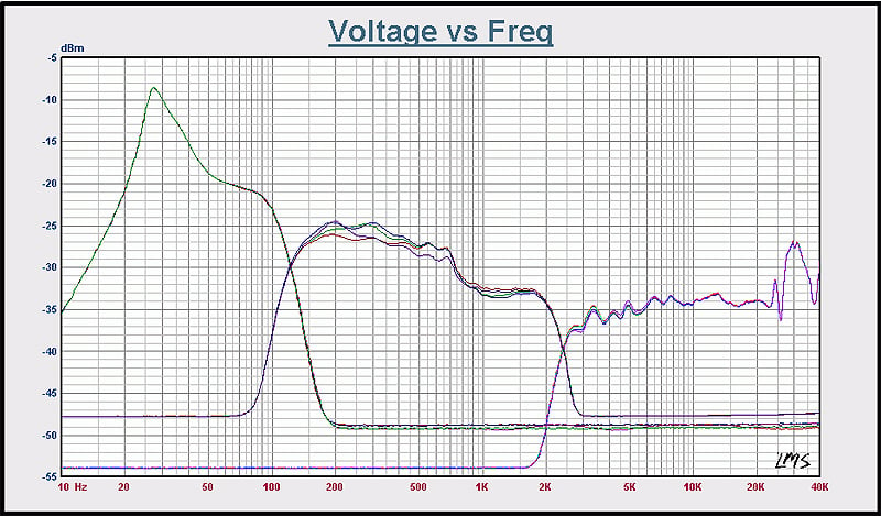
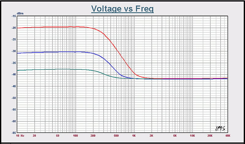
Figure 3a, b: A: XdA Out; B: XdW Amp Out
Curious to see just what the XdA’s output looked like, the voltage vs. frequency curves seen in Figure 3a were generated. At left (in green) in Figure 3a is the XdA balanced out to XdW response. The collection of curves seen in the middle is the XdA’s output to the XdS midrange driver as presented when each of the 4 output modes are activated. The collection of curves showing at right in Figure 3a is, of course, for the XdS tweeter. Note the minimal effect seen by switching modes on the tweeter’s magnitude response plots. Taking into account the complexity of the individual curves its easy to appreciate the complexity of the task handed the XdA’s DSP functions.
Curious to see what, if any, role in contouring the XdW’s amplitude response plot was played by the XdW’s built-in power amplifier, the voltage vs. frequency curves seen at right in Figure 3b were generated. The frequency sweeps were done at the “More” (red), “Just Right” (blue) and “Less (green) levels. As can be seen, there is indeed some low-pass contouring going on, varying with however the XdW’s trim is set.
NHT XdS Conclusion
The NHT Xd system is the successful realization of an ambitious technical goal NHT set for themselves years ago. It’s a brilliant melding of disparate technologies that so well expresses itself with musical elegance, finesse & power. Critical listeners everywhere will experience musical satisfaction to an altogether uncommon depth & degree. Forward looking, yet firmly rooted in the time-tested basics of system design, the Xd is a system whose whole is much greater than the sum of its well-engineered parts. Both aesthetically and sonically this system is a trend setter and is likely the leading edge of more DSP-controlled, Class D-powered systems that will follow in its footsteps. This system comes highly recommended to those who demand both sonic excellence and a product that adds a strikingly attractive new dimension to the overall visual appeal of their listening space. Be sure to get a copy of the sampler disk, too.
NHT
6400 Goodyear Road
Benicia, California
94510
http://nhthifi.com
Phone: 1-800-NHT-9993
The Score Card
The scoring below is based on each piece of equipment doing the duty it is designed for. The numbers are weighed heavily with respect to the individual cost of each unit, thus giving a rating roughly equal to:
Performance × Price Factor/Value = Rating
Audioholics.com note: The ratings indicated below are based on subjective listening and objective testing of the product in question. The rating scale is based on performance/value ratio. If you notice better performing products in future reviews that have lower numbers in certain areas, be aware that the value factor is most likely the culprit. Other Audioholics reviewers may rate products solely based on performance, and each reviewer has his/her own system for ratings.
Audioholics Rating Scale
 — Excellent
- — Very Good
- — Good
- — Fair
- — Poor
| Metric | Rating |
|---|---|
| Build Quality | |
| Appearance | |
| Treble Extension | |
| Treble Smoothness | |
| Midrange Accuracy | |
| Bass Extension | |
| Bass Accuracy | |
| Dynamic Range | |
| Performance | |
| Value |