
Denon AVR-3806 Audyssey MultEQ XT Test Report
Audyssey’s MultEQ XT is a sound equalization system that’s finding its way into more and more audio-related products destined for the consumer electronics marketplace. Its encapsulated on a TI Aureus chip, found in Denon flagship products or in the case of the Denon AVR-3806 and other brand products , an Analog Devices’ chip. Based on research originally carried out under a National Science Foundation grant at USC’s Integrated Media Systems Center, MultEQ XT represents a nonlinear signal-processing approach to the substantial challenge of room response equalization.
Traditional approaches to EQing typically featured time or frequency domain measurements of the room response made at a single (or multiple) listening position(s) and deriving from the results a filter (EQ) response that’s an inverse of the room response. Mathematically, the traditional approach looks like:
Where: 
heq (n) = filter (EQ) response
h (n) = room response
Convolution operator
δ (n) = 1 (for perfect equalization); Kronecker delta function

Or looked at another way (RMS average):
where: 
Here,  , is the magnitude
response at position i.
, is the magnitude
response at position i.
Seems simple enough, but given the complex nature of room acoustics, the traditional approach is a dicey proposition that frequently leads to disappointing results: often requiring considerable subsequent tweaking by ear before arriving at a compromise solution. The “solution” may nevertheless work only for one listening position, if at all. When considered that a linear, electronic device, operating in the frequency domain (your EQ) is being asked to provide a solution to what is largely a non-linear, time-domain problem of an acoustical nature, uncertain, disappointing or otherwise inconsistent outcomes aren’t entirely surprising.
The approach Audyssey has taken - embodied in the MultEQ XT system - is to consider this formidable equalization problem as one of pattern recognition. (Now there is an original approach!) Through the application of a Fuzzy-c means clustering algorithm applied to the raw data gathered during measurement, an equalization solution is found by way of a three-step process: (1) Prototypical representations of room responses are derived from collections of room measurements grouped in clusters, clustered according to their degree (or lack of) similarity; (2) the prototypical responses are further combined, forming a general point response; and (3) the minimum phase component of the general point response is inverted resulting in the required equalization filter response. The process is driven by a target function, which is a pre-determined “ideal” amplitude response curve to which the MultEQ XT attempts to design a best-fit equalization solution.
Editorial Note on Fuzzy-c means ClusteringClustering, generally speaking, is the process of grouping raw data (in this case, measured room responses) into homogenous clusters having centroids (analogous to a center of mass) or prototypes. Fuzzy-c means clustering is an overlapping, non-hierarchical clustering approach that allows one piece of data to belong to more than one cluster. (The term “fuzzy” relates to how the raw data are bound to any particular cluster by a continuous membership function). Fuzzy clustering assigns degrees of membership of the various measured room responses to appropriate clusters by way of the previously mentioned continuous membership function. The degree of similarity between measured room responses determines the degree of membership held by any particular data in any particular cluster. Mathematically, the Fuzzy c-means algorithm for determining the cluster centroids looks like:
;
Where:
ith cluster room response prototype
continuous membership function
dik = the Euclidean distance between the room responses at positions i and k, respectively.
The goal here is to create a magnitude response, minimum-phase, equalization filter based on a final room response prototype. This final prototype response is actually a linear combination of all cluster centroids under consideration. This step in the process is accomplished by the application of a non-uniform weighting model:
The required filter is obtained by inverting the minimum phase component,
of the final (centroid) prototype,
. (The minimum phase component is found from the cepstrum of
).
The level of activation of any particular prototype will depend on the degrees of assignment of the measured room responses to the cluster containing the prototype. The final prototype is formed by a nonuniform weighting of the cluster membership function such that the more dense a cluster (in terms of the fuzzy membership function) the greater the contribution will be made by the corresponding centroid in forming the final prototype, with a parallel increase in the effect had on the final multiple-position EQ filter.


Mathematically speaking, MultEQ XT certainly looks good. Now let’s put the system through its paces and see what the amplitude response measurements have to show.
Audyssey Set-Up and Calibration Process
Setting up the MultEQ XT system was fairly straightforward and took, in this particular case, about 10 minutes to complete.
The process begins with placement of the Denon mic at the main listening position, M1, (see Figure 1), positioned at a height approximating the ear height of a seated listener. MultEQ XT depends, by design, on the first measurement run being made at the main listening position. Therefore it is critical the process commences with the Denon mic located at no spot other than M1, wherever that may be in your listening room. A series of repeated test signals are then generated from which the processor gathers its initial calibration data, such as number of speakers, speaker type (sub or satellite), component polarity, and optimal crossover frequency. It then calculates individual speaker-to-mic distances, setting delay & trim for each channel. If the MultEQ XT discovers any problems at this stage, it will let you know that, too. For example, MultEQ XT might find a component opposite in absolute polarity to all the rest. This might be a case of reversed leads or an intended design feature (not uncommon in 3-way loudspeaker systems). Incidentally, MultEQ XT doesn’t care what the polarity of any particular component might be; it merely presents its findings for your use. It has no effect on subsequent calculations.
Once this initial stage is complete, the end-user then moves the measurement microphone to the remaining 5 positions, M2 – M6. At each step a series of test signals are again generated; measurements are made and when completed the mic is moved to the next position, the process repeated until measurements have been completed at position M6. The raw time domain data generated by the collection of measurements provide the building blocks from which the patterns mentioned in the above editorial note are identified. Subsequently an equalization solution, based on a target function, is found and stored. At that point the little green light on the front of the AVR’s faceplate goes on indicating MultEQ XT is active and its all systems go!
Figure 1 illustrates the general layout of the listening room where the measurements were made along with the disposition of the already-mentioned 6 measurement points required by the MultEQ XT system, as implemented in the Denon AVR-3806. (The blue block lines are theater drapes). If you have theatre-style seating and the chair backs can be dropped, the recommended practice is to drop the backs, place the Denon mic, as mentioned earlier, at a height equivalent to listener ear height (or the default 1m) over each seat and measure away. In this case, because the couch back couldn’t be dropped, rather than hang the mic(s) over the couch, I moved the couch out of the way, did the MultEQ XT setup, then moved the couch back into the area for which MultEQ XT had been set up.
The placement pattern was dimensioned approximately one couch wide and two seat rows deep. Try not to cluster the measurement spots too closely otherwise you run the risk of providing MultEQ XT with insufficient low frequency information. The one exception to this recommended practice might be the case where you’re dealing with a highly directional loudspeaker system(s) or a system exhibiting extremely pronounced off-axis lobing. In either case MultEQ might interpret the incoming signal as being indicative of diminished HF content and jack the gain in that part of the audible spectrum, resulting in a system with a hot high end.
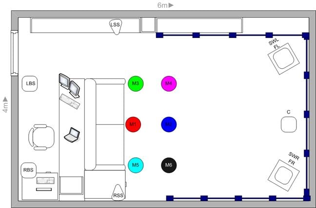
Figure 1: Room layout and measurement mic disposition. Note for this series of tests the subs were place directly beneath the front L & R speakers.
Figure 2: Mic positions determined by laser pointers (note red dots).
A series of before/after measurements were made at each of the 6 measurement positions. To be certain that the measurement mics always returned to the same point in space occupied by the Denon-supplied setup mic, a pair of laser pointers were used for positioning .For all measurements, the mics were positioned .83m (~33”) from the floor (average ear height for listeners seated on the couch) . Note that the Denon-supplied calibration mic seen at left in Figure 2 is pointed upward. The mic calibration file hard-coded in the AVR was derived with the mic oriented vertically and requires the mic be positioned likewise when in use. Doing otherwise (eg: pointing it directly at the center speaker) increases the risk of bogus results. Because each calibration is unique to the mic from which it was derived, it is essential that no mic other than the one that shipped with the AVR be used: doing so, once again, increases the risk of bogus results.
Note too that a mic stand was used to position both the Denon and measurement mic. Using a mic stand or at the very least a tripod is the correct approach. Placing the Denon mic on the seat or back of chair/couch or simply holding the thing in your hand can significantly alter the mic’s perception of the incoming acoustic signal, likely causing – you guessed it – bogus results.
Editorial Note on Measurement Mics
If you’re interested in measuring for yourself the effects MultEQ XT has on your system, a caution is in order regarding the mic you make the measurements with.
The LinearX M31 mic used to record the various amplitude response plots featured in this article is oriented vertically, pointing upward towards the ceiling. This is a commonly recommended orientation for the sort of measurements done here. However, the calibration file supplied with the M31 assumes a free-field frequency response to sound waves that are at normal incidence (perpendicular) to the mic’s diaphragm. That is to say, the validity of the calibration is based on the assumption that the mic is pointed directly at the loudspeaker(s). With the microphone rotated 90°, that assumption is no longer entirely valid and a second calibration file is required to maintain accuracy. This second calibration file assumes a pressure-field frequency response to sound waves that are now parallel to the mic’s diaphragm. Just how and where the M31’s frequency response is affected by this change in orientation can be seen by looking at the differences in the required calibration curves, illustrated in the figure below.
M31 free-field (blue) and pressure-field (red) calibration curves.
The two separate calibration curves needed in order to maintain measurement accuracy doing free- or pressure-field measurements can be seen to diverge, beginning ~ 2.5kHz. In actual use, orienting the M31 vertically without using the red pressure-field calibration curve results in response plots that appear to roll off at the HF end of the audible spectrum much more quickly than they actually are, effectively rendering the measurements inaccurate. Herein lies the caution: where required, use the correct calibration file for the type of measurement you are performing!
Denon AVR-3806 Audyssey MultEQ XT Test Report (cont)
Figure 3 is a collection of pre-MultEQ XT amplitude response plots as measured at M1 – M6. (Note: the M dots in Figure 1 are color-coded to coincide with the plot colors in Figure 3, along with all other graphs where individual response plots are featured). The room’s modal structure, evidenced in the individual plots, had its anticipated effect; made up of both peaks & dips, the picture presented indicated a formidable challenge for the MultEQ XT! I was especially curious to see what the MultEQ XT system would do with the peak at ~ 25Hz as well as the dip at ~ 50Hz that persisted across each of the 6 measurements.
Figure 3: Pre-MultEQ dB spl Amplitude Response plots (1/12th Octave Smoothed) As
Measured At Listening Positions M1, 2, 3, 4, 5, & 6
Figure 4 is the response plot resulting from averaging all 6 pre-MultEQ measurements together. This will be used later for comparison with both the averaged post-MultEQ XT plots, as well as the hard-coded MultEQ XT target function. Doing so will clearly illustrate the effect MultEQ XT has on the system’s amplitude response.
Figure 4: Vector RMS Average of Pre-MultEQ XT dB spl Response Plots As Measured At
Listening Positions M1, 2, 3, 4, 5, 6
Figure 5: Post-MultEQ XT dB spl Amplitude Response Plots (1/12th Octave Smoothed) As
Measured At Listening Positions M1, 2, 3, 4, 5, & 6
The MultEQ XT process was then run to completion and the post measurements were made.
In Figure 5 we see the post-MultEQ XT amplitude response plots generated measuring, once again, at positions M1 – M6, color coded as before. Figure 6 is the result of averaging all 6 measurements together. Cursory examination of Figs. 3 – 6 shows changes have indeed occurred.
Overall, it would appear the individual post-MultEQ XT plots have tightened, becoming more alike or similar in appearance than their pre-MultEQ XT counterparts. In fact, they now more closely resemble the hard-coded target function mentioned earlier.
As well, it can be seen that the LF peak at ~ 25 Hz remains, but has been somewhat tamed. So too has the dip: frequency-wise shifted downward a bit, but otherwise largely remains untouched. The fact the LF dip remains is important as it indicates the MultEQ system wisely did not attempt to pointlessly fill it with extravagant amounts of LF acoustical energy. There are other means to deal with the dip; experiment with sub placement prior to running MultEQ XT for best results.
Given the practical constraints arising from packing FIR filters with sufficient numbers of taps (necessary for dealing with low frequency signals) into a DSP already running other processes, an approach whereby resolution varies continuously with frequency was employed. The net result is that at low frequencies (say, below 100 Hz) MultEQ XT could more effectively deal with .5 Octave wide peaks than a .083 Octave wide peak.
Another interesting feature is the appearance of an upswing at approximately 25kHz in both post-MultEQ XT plots. It’s the LMS system picking up the acoustic output of a motion-detection system that happened to be operating nearby. Its actually been part of all the measurements taken, though not until the MultEQ XT system took over was it visible in the amplitude response curves.
Where it comes to background noise, it pays to heed all warnings relating to keeping things quiet while the MultEQ XT system is progressing through its measurement sequence. Because a substantial signal to noise ratio is required to successfully complete the sequence, the overall background noise floor must be kept low otherwise the process stops and MultEQ XT throws an error message
It appears the nature of the noise may have some bearing on how MultEQ XT deals with it. When I first put the system through its paces, quite a lot of LF acoustic energy from the air-handling system bled through, convincing MultEQ XT that a large segment of the subwoofer’s output was at a significantly higher amplitude than it actually was. The end result was MultEQ XT applied the brakes and pretty much wiped out much of the lower portion of the sub’s output. For this sequence of measurements, steps were taken to ensure air handler noise did not intrude. No further problems were encountered.
Figure 6: Vector RMS Average of Post-MultEQ XT dB spl Response Plots As Measured At
Listening Positions M1, 2, 3, 4, 5, 6
As mentioned earlier, MultEQ XT calculates speaker-mic distance for each of the individual system components during the initial calibration stage of the setup sequence. Figure 7 compares the actual measured distance (from the center of each loudspeaker’s faceplate to mic tip center) with that calculated by MultEQ XT. The figures are in fairly good agreement, in each case the MultEQ XT distance is longer than the measured distance, in part owing to driver voice coil-to-faceplate offset. The voice coils are, of course, recessed relative to the respective cabinet’s faceplate and are thus slightly more distant from the mic than the faceplate.
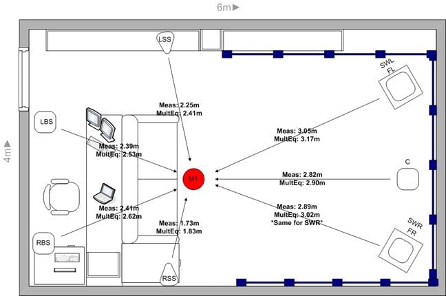
Figure 7: Component distance (m) Measured vs. MultEQ XT-determined
MultEQ XT also configures speaker size and crossover frequencies. Any speaker, exhibiting a -3dB point measured at or above 80 Hz is designated as “Small”. Conversely, those measuring a -3dB point below 80 Hz are designated as “Large”. Occasionally, boundary gain can result in a “Small” being designated as “Large”. Figure 7b is a screen capture showing MultEQ XT's crossover frequency speaker size choices.
Figures 7b: MultEQ XT-determined Crossover Frequencies
Audyssey determines speaker size based on whether a particular speaker’s -3dB point falls above or below 79 Hz. (Should MultEQ XT estimate speaker size, speaker distance, crossover frequency or channel trim wrong, the settings can be manually tweaked later, if needed).
Finally, Figs. 8 & 9 give us a look at just what the MultEQ XT system did for the overall system amplitude response, as measured across the listening area.
Figure 8 shows the pre- & post-MultEQ XT averaged response plots. Its clear the MultEQ XT system has had an effect on the amplitude response, particularly in the 200Hz – 2kHz range. Figure 9 is Figure 8 repeated but with 1/3rd Octave smoothing employed to enhance visual clarity and the hard-coded target function overlaid, giving a better visual sense of how successful the MultEQ XT was in pulling the system’s overall response closer to that of the target function. Once again, it can be seen that the MultEQ XT system did manage to polish the response. This can best be seen in the blue trace below in the smoothing out of the 60 Hz and 150 Hz regions, as well as cutting a peak at around 250 Hz, filling a hole at 1.2 kHz and lowered the nasty peak at 30 Hz. The MultEQ XT correction helped to bring the response in line as something closer to the target function than the pre-MultEQ XT amplitude response.
Figure 8: Vector RMS Average of Pre- (Red) and Post- (Blue) MultEQ XT dB spl Response Plots
As Measured At Listening Positions M1, 2, 3, 4, 5, 6. Data 1/12th Oct Smoothed
Figure 9: Vector RMS Average of Pre- (Red) and Post- (Blue) MultEQ XT dB spl Response Plots
As Measured At Listening Positions M1, 2, 3, 4, 5, 6. With MultEQ XT Target
Function (Purple) Overlay Data. 1/3rd Oct. Smoothed
So how did it sound?
The overall tonal balance of the system did change, but only modestly so. There were, however, other much more noticeable changes that had occurred. Foremost was a widened sweet-spot with enhanced clarity, imaging and localization across the now seamless, 3D soundstage. In effect, it appeared the center of the original sweet-spot had spread to cover 6 different listener positions! Not bad.
The Denon 3806 AVR offers four room EQ options, Audyssey (MultEQ XT), Front, Flat, and Manual.
-
“Audyssey”: we already know about.
-
“Front”: was included to satisfy an early licensee’s requirement that while the MultEQ XT process was applied, the front L & R speakers would otherwise remain untouched, filterwise. (The idea being that people with very expensive, high-end fronts wouldn’t want them touched by any equalization). In this case MultEQ XT averages the amplitude response of the fronts and uses the resulting curve as the target function applied to equalizing the remaining speakers.
-
“Flat”: essentially identical in form & function to “Audyssey”, with the exception being there is no high end roll-off (as seen in the purple target curve appearing in Figure 9.) “Audyssey” and “Flat” are likely the most commonly chosen options. Good first choice for listening to music.
-
“Manual”: isn’t part of the Audyssey MultEQ XT process and is a final option that provides for a simple, manually-operated graphic EQ. (See figure below).
 The degree to which the MultEQ XT system will
enhance a system’s performance depends on a number of factors and any
particular listener’s experience will likely be different from that of
another’s. The overall intrinsic quality of the AVR/loudspeaker components as
well as the location of the loudspeakers themselves are probably the leading
factors determining just how and to what degree MultEQ XT will effect the
system’s overall performance. All in all the inclusion of the MultEQ XT system within
an AVR destined for home use is a worthwhile addition and a successful step
forward in bringing audio nirvana to the home theatre.
The degree to which the MultEQ XT system will
enhance a system’s performance depends on a number of factors and any
particular listener’s experience will likely be different from that of
another’s. The overall intrinsic quality of the AVR/loudspeaker components as
well as the location of the loudspeakers themselves are probably the leading
factors determining just how and to what degree MultEQ XT will effect the
system’s overall performance. All in all the inclusion of the MultEQ XT system within
an AVR destined for home use is a worthwhile addition and a successful step
forward in bringing audio nirvana to the home theatre.
Bibliography
1. Y. Haneda, Y., Makino, S., Kaneda, Y,: “Common Acoustical Pole and Zero modeling of room transfer functions”, IEEE Transactions on Speech and Audio Proc.,vol. 2(2), pp. 320{328, Apr. 1994.
2. Bharitkar, S. & Kyriakakis, C.: “A Cluster Centroid Method For Room Response Equalization At Multiple Locations” WAASPA 2001, New York 2001
3. Bharitkar, S. & Kyriakakis, C.: “New Factors in Room Equalization Using a Fuzzy Logic Approach” Audio Engineering Society, Convention paper, 111th Convention, New York, Sept. 2001
4. Bharitkar, S. & Kyriakakis, C.: “Perceptual Multiple Location Equalization With Clustering” 36th IEEE Asilomar Conference on Signals, Systems, & Computers, Pacific Grove, CA, Nov. 2002
5. Bharitkar, S. & Kyriakakis, C.: “Visualization of Multiple Listener Room Acoustic Equalization with Sammon Map” IEEE Transactions On Speech And Audio Processing
6. Bharitkar, S. & Kyriakakis, C.: “The Influence of Reverberation On Multichannel Equalization: An Experimental Comparison Between Methods”, 37th IEEE Asilomar Conference on Signals, Systems, & Computers, Pacific Grove, CA. Nov. 2003
7. Allen, J.B. & Berkley, D. A.: “Image method for efficiently simulating small-room acoustics”, Acoustics Research Department, Bell Laboratories, Murray Hill NJ, June 1978
8. Bharitkar, S. & Kyriakakis, C.: “Multirate Signal Processing for Multiple Listener Low Frequency Room Acoustic Equalization”, Proc. 2004 38th IEEE Asilomar Conference on Signals, Systems, & Computers. Pacific Grove (CA). Nov.2004
9. Bharitkar, S., Hilmes, P., & Kyriakakis, C.: “Sensitivity of Multichannel Room Equalization to Listener Position”, Audio Engineering Society Convention Paper, 115th Convention, October 2003, New York
10. Bharitkar, S., Hilmes, P., & Kyriakakis, C.: “Sensitivity of Multichannel Room Equalization to Listener Position”, Audio Engineering Society Convention Paper, 115th Convention, October 2003, New York
11. Kyriakakis, C.: “Fundamental and Technological Limitations of Immersive Audio Systems” Proceedings of The IEEE, Vol. 86, # 5, May 1998
12. Bharitkar, S., Hilmes, P., & Kyriakakis, C.: “Low Frequency Robustness of Multiple Listener Equalization with Magnitude Response Averaging”, Audio Engineering Society, New York
13. Oppenheim, A., Johnson, D., Steiglitz, K.: “Computation of spectra with unequal resolution using the fast fourier transform” Proc. IEEE, 59, pp. 299-301, 1971.
14. Mourjopoulos, J.: “On the variation and invertibility of room impulse response functions” Journal of Sound and Vibration, Vol. 102 (2) pp. 217-228, 1985
15. Kosko, B.: “Fuzzy System as Universal Approximators”, IEEE Trans. on Neural Networks, Vol. 43(11), pp. 1329-1333, Nov. 1994
16. Haneda, Y., Makino, S., & Kaneda, Y.: “Common Acoustic Pole and Zero modeling of room transfer functions” IEEE Transactions on Speech and Audio Proc., Vol. 2(2), pp. 320-328, Apr. 1994
17. Bezdek, J., “Pattern Recognition with Fuzzy Objectiver Function Algorithms”, Plenum Press New York. 1981
18. Beni, G., Xie, X. L.: “A validity measure for fuzzy clustering”, IEEE Transactions on Pattern Analysis and Machine Intelligence, Vol. 3, pp. 841 – 846, 1991.
19. Denon: “AV Surround Receiver AVR-3806 Operating Instructions”, Denon Brand Company, D & M Holdings, Inc., Tokyo, Japan
20. Bruel & Kjaer: “Microphone Handbook, Vol. 1: Theory”, Technical Documentation, BE 1447-11, Brüel & Kjær, Naerum, Denmark
21. Bruel & Kjaer: “Condenser Microphone Cartridges – Types 4133 to 4181”, Product Data Sheet, BP 0100 – 17, Brüel & Kjær, Naerum, Denmark