
Five (5) Audio Myths Dispelled
originally published on AudioXpress
In my spare time I've been known to peruse various websites, newsgroups and other online forums devoted to all things loudspeaker. Over the years I've learned quite a bit; gaining further insights into the art & science of speaker building from both luminary and amateur enthusiast alike. And if you, like me, spend any time following the variegated tracery of threads which make up these various online resources, you'll also know the noise-to-useful-information ratio can be very large indeed.
I've seen it happen often where an idea or concept, lacking little or no technical merit or validity is promulgated as truth. And those seemingly invincible items that pop up year after year, I've elevated to the rank of "myth". I've taken look at some of my favorites under the objective light of hard science and I'd like to share the outcome of my own investigation into these favorite myths of mine.
The Five Myths that will be covered in this article include:
1. Damping Factor
2. Magnetic Shielding
3. Gold is the Best Conductor
4. Bass Reflex Is More Efficient Than Totally Enclosed Box
5. The Perfect Driver
1. Damping Factor
Quite a large amount of online text has been devoted to this item in the forums I mentioned earlier. Reading the various discussions raging back and forth between contributors, the general sense I get is most folk attribute to the contribution to total system damping factor made by an amplifier - and its effect on system performance - far more than should be.
Damping Factor (DF) is defined as the ratio of the load impedance (usually taken as 8 ohms) to source impedance. It is a dimensionless figure of merit and therefore has no units ascribed to it. In practical terms, when applied to an amplifier, it indicates to what degree the amp can dissipate the energy generated by a driver's voice coil as the coil's post-impulse motion decays to zero: thus is the mechanical vibration electrically damped. But focusing solely on DF as determined by an amplifier's output resistance (Rg) is too narrow in scope as it's Rsource, the sum of Rg, cable resistance (Rcable), crossover network component resistance (Rcomponent) and Revc (voice coil resistance) that determines the true DF as seen by the driver. Focusing on Rg alone also ignores the single largest contributor to DF: the driver's voice coil.
To get a clearer picture of DF and its effect on system performance, I ran a series of simulations to determine to what degree various damping factor values as determined by Revc, Rg, Rcable and Rcomponent affect system response performance at resonance frequency.
In the first simulation set I ran I used a test model representing a closed-box system, whose initial design was based upon DF = ∞, Rsource = 0 Ω, where:
Rsource = Rg + Rcable + Rcomponent (Ω)
and a Qtc = 1/√(2), (Butterworth B2 alignment) producing a maximally-flat response, with zero peak at resonance. Although DF is typically specified at a load impedance value of 8 Ω, for my calculations I used Revc = 6.2 Ω, which was the Revc parameter value of the driver I modeled (KEF B139). If you're more comfortable thinking of DF in terms of the usual 8 Ω load, you can convert the given 6.2 Ohm-based Rg figures to 8 Ω based values by multiplying the given values by 1.2903. At any rate, in running the analysis, some interesting trends emerged from the data generated by the simulations.
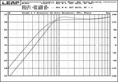
Fig 1: System response at DF = 1 and DF = ∞
As mentioned earlier, the Rg or amplifier output resistance, in actual practice is only part of Rsource, all three components of Rsource, along with Revc, combine to affect DF. Of all resistance components, however, Revc is by far the largest and therefore has the greatest effect of all on DF. For now, let's focus on Rg alone.
Rsource affects system response by affecting Qec, which in turn affects system Qtc. Rewriting the well-known formula for calculating Qtc from Qec and Qmc, but taking into account Rg, Revc, Rcable and Rcomponent gives:

Where:
Qec' = System Q at resonance (fc), due to electrical losses, including Rsource, dimensionless
fc = System resonance of Totally enclosed box (TEB), Hz
Bl = Force factor, Magnetic flux density in voice coil gap * coil winding length, TM
Rsource = Rcable + Rcomponent + Rg (Ohms)
Plugging Qec' (which represents Qec modified to take into account Rsource) into the well-known equation
used to calculate Qtc
Where:
Qtc' = Total system Q at resonance (fc) due to both mechanical and electrical losses, taking in to account Rsource, dimensionless
Qmc = System Q at resonance (fc), due to mechanical losses, dimensionless
A cursory examination of these formulae shows that as Rg increases, so too does Qtc and with the increase in Qtc comes an increasing response peak at resonance. And, of course, adding the other two components that make up Rsource, Rcable and Rcomponent, combine to produce even larger changes in Qec, Qtc and system response at resonance.
The question is, at what point does the affect of declining DF becomes audible? Looking at the first dataset, which I generated considering Rsource, it would appear that only in the very worst of cases do these changes enter the realm of possibly audible. And setting the upper value limit of Rsource = Revc is certainly an extreme case!
Fig 2: DF, Rsource and resulting variations in Electrical attenuation, Resonance Peak and Qtc'
|
DF Elec. Attn. (dB) Rsource (Ω) Resonance Peak (dB) Qtc' |
|
∞ -20 * Log (∞) 0.0000 0.00000 0.7071 |
|
1000.0 -60.000 0.0062 0.00000 0.7075 |
|
500.0 -53.970 0.0124 0.00000 0.7079 |
|
100.0 -40.000 0.0620 0.00060 0.7116 |
|
50.0 -33.979 0.1240 0.00270 0.7161 |
|
20.0 -26.020 0.3100 0.01580 0.7295 |
|
15.0 -23.520 0.4133 0.02717 0.7368 |
|
10.0 -20.000 0.6200 0.05676 0.7512 |
|
5.0 -13.979 1.2400 0.18422 0.7925 |
|
2.0 -6.020 3.1000 0.69477 0.9013 |
|
1.0 0.000 6.2000 1.50960 1.0447 |
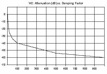
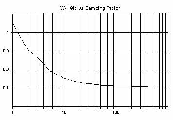
Fig 3: Attenuation (dB) vs. Damping Factor
Attenuation = -2.5286e-005 - 8.6851 * ln (DF)
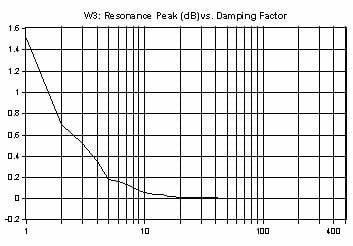
Res. Peak = (0.4094 + 0.3988 * DF) ^ (-1/0.5171)
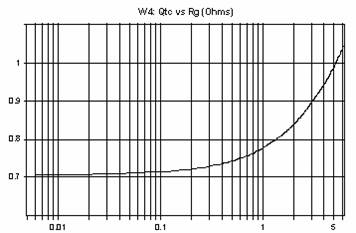
Fig 5: Qtc vs. Rg (Ohms)
Qtc = (0.7070 * 17.4457 + 1.9938 * Rsource ^ 1.0005)
Qtc = 1.3499 - 0.6422 * exp (-0.7349 * DF ^ - 1.0303)/ (17.4457 + x ^ 1.0005)
Looking where in the Qec' equation that Rsource is positioned tells us that keeping it as low as possible is helpful, but only modestly so given that Revc, under typical circumstances, is much, much larger.
This is key to understanding the true nature of DF is it's the total resistance seen by the driver's motor coil that counts and that Revc is, by far, the largest, single most important contributor to the total resistance value of the amp/cable/component/voice coil circuit. Because the value of Rsource tends to be < < Revc, Rsource doesn't change all that much the degree of damping the driver experiences at resonance owing to its own Revc. Why?
Damping is energy dissipation; here in the form of direct conversion of electrical power into heat, with the end result said energy is no longer stored in the system. Typically, 95%+ of the power supplied by the amplifier winds up as heat generated by the voice coil.
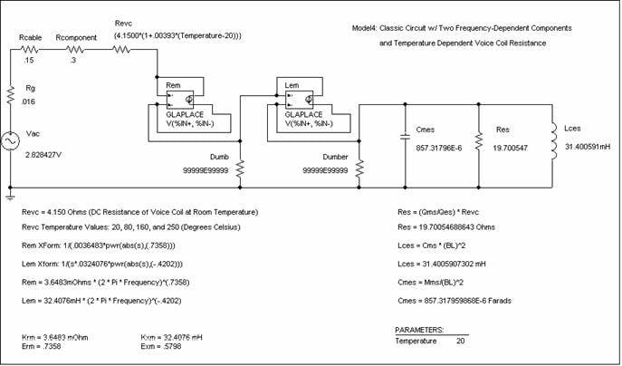
To get a clearer picture where and to what degree dissipation occurs within the amp/cable/component/voice coil circuit, I ran a simulation of a driver based on a circuit, the schematic of which some of you may recognize as one I presented in an earlier Speaker Builder article.
In that article, I demonstrated how to create an accurate model (with both temperature and frequency dependent components) of a raw driver using PSPICE. I've added Rg, Rcable and Rcomponent values, retaining the original model Revc value of 4.15 Ohms, found in that earlier article. I then probed for power dissipation at each of the 4 components to see how and where power was being dissipated.
For those who'd like to experiment with the model using their own circuit editor/analyzer, I've included the netlist generated by PSPICE.
Fig 7: SPICE Net list For Test Circuit
Fig 8: Test Circuit
Once the simulations were run it was easy to see from the generated output graphs that, indeed, the majority of dissipation - and therefore damping - was taking place in the Revc component of the circuit, i.e., the driver's voice coil. In the graph, the topmost trace is that of Revc, which clearly indicates Revc is that point in the circuit is where the most power is being dissipated.
Fig 9: Power dissipation amongst the Rsource components
 Hence, it has the greatest degree of control in determining the DF of the circuit.
By this point in the analysis it should be clear, where it comes to DF that real control lays with the driver's voice coil Revc and not with Rsource. However, there is another reason for keeping Rsource as low as possible. That's found in looking at its effect on something entirely separate from DF: dB SPL loss, where:

Here, Zevc represents the frequency-dependent impedance of the driver's voice coil, in Ohms. This equation illustrates that increasing Rsource results in greater dB SPL losses. Given this fact, best practices dictate keeping Rsource as low as possible.
From my preceding investigation I think it fair to draw the conclusion that amplifier DF has very, very little effect on the total circuit DF and what little effect it does have occurs only in the very worst of cases.
For more related reading material on Damping Factor, check out: Damping Factor: Effects on System Response
2. Magnetic Shielding
These online threads typically start with someone bemoaning the fact that their latest design, now made reality, can't be placed next to their TV or CRT computer monitor without making the display go all distorted. What to do?
Soon follows lots of well-intentioned suggestions - frequently possessing scant traces of technical merit - to shield or enclose the monitor or loudspeaker with a variety of metals. To sort the rubbish from the useful suggestions, I ran a series of Finite Element Analysis (FEA) analyses, each modeling a different suggestion on how to conquer video display distortion. My analyses will show, in the end the old saw "ounce of prevention is worth a pound of cure" definitely holds true where it comes to effectively corralling stray magnetic fields.
 The first simulation is that of a magnet\steel structure with its magnetic field free to fill the air surrounding it. The squiggly lines surrounding the structure are magnetic field lines, scaled in Webers. Any electrons streaming through the magnetic field (such as those found in an energized cathode ray tube) will be pulled off course, resulting in all sorts of image distortions.
One solution, of course, is to keep that magnetic field from getting near the electron path. Moving the field source a sufficient distance from the CRT gun would clear things up as the farther the distance from the source the lower the flux density, but that only addresses the symptoms, not the underlying pathology. As well, practical space constraints may make putting enough space between monitor and speaker impractical.
For my second simulation, I modeled another common suggestion: place a shield between the loudspeaker and the CRT. In this case I placed a sheet of aluminum squarely in the path of the field and it did … just about nothing. Look at those lines - they're having a field day!
Fig 10a: Unrestrained Magnetic Field
 This looks like a sure-fire formula for disappointment, so obviously it isn't a useful solution. The problem here is that aluminum is a non-ferromagnetic material with a relative permeability value nearly identical to that of air - thus its about as useful as air in corralling the stray magnetic field and preventing CRT image distortion. Display distortion continues virtually unabated.
Fig 10b: Magnetic Field With Aluminum Shield
 For my third simulation I modeled another common suggestion: enclose he loudspeaker in a container of some sort. In this case I used copper as the material. Once again we see the field is anything but corralled, which is just what we would expect using yet another non- ferromagnetic material.
Copper has a relative permeability very close in value to that of aluminum and the results from this FEA run reflect this. Both aluminum and copper have permeability values nearly that of air and thus these non-ferromagnetic materials have no real ability to redirect lines of flux. Any CRT caught within the field surrounding the copper box would suffer distortions just as it would with the aluminum shield modeled previously.
Once again, display distortion continues.
Up to this point I've modeled "cures" that address the symptoms but none of which do a thing towards resolving the underlying pathology. It could reasonably be argued that other materials such as steel, mumetal, etc, could have been used to create the modeled enclosure. But their effectiveness, practicality, predictability of results, etc, when measured against cost and so forth still don't make it worthwhile, especially when addressing the underlying pathology in the first place is proven solution: effective, predictable and comes with an added bonus as well.
Fig 10c: Magnetic Field With Copper Box
Besides, suppose you did find a material that could effectively control the shield the CRT monitor from the magnetic field surrounding the loudspeaker system. You'd need to enclose the entire system in the metal I order to maximize effectiveness. And who wants to listen to a loudspeaker entirely contained within a metal box? Not very practical.
 In my fourth FEA simulation I modeled the magnet structure with a second magnet (also know as a bucking magnet) of the correct size, shape, material and orientation placed up against the original magnet structure.
Here we can see that the magnetic field is very effectively corralled, certainly far better than obtaining in any of the preceding simulations.
Best practices here dictate that using drivers with a built-in bucking magnet already in place is the correct way to prevent CRT- distorting magnetic fields getting at your TV or computer monitor.
The bonus? The presence of the bucking magnet can increase field density in the voice coil gap, which, in turn means increases efficiency and lowered Qes, as compared to its non-bucking equipped twin. Conversely, placing a cup shield made out of a ferromagnetic material around the magnet assembly will typically result in a reduction in field gap density, which results in reduced Bl, efficiency and increased Qes - all because the cup provided a lower reluctance path for the flux to follow than that obtaining within the voice coil gap.
Fig 10d: Magnetic Field With Bucking Magnet
In all, analysis shows that its better to avoid the problems created by stray magnetic fields when your system needs to be placed near a CRT monitor by using drivers built with the bucking magnet already in place, rather than attempt to devise a shield of one sort or another.
3. Gold is the Best Conductor
Often found buried in online discussions of cables and interconnects is the contention that Gold is the best conductor from which to make said items. Reality is, whether or not gold (or any other metal, for that matter) is the best choice of conductor depends on the application for which it is intended.
I've put together a chart listing basic properties of several metals I've seen mentioned at one time or another in online discussions. From a material properties point of view, gold's most outstanding feature is that it's a noble metal and therefore does not react with the environment as the other metals do, which makes it a
great choice for corrosion-resistant connectors.
A quick look at the chart show its not the least resistive or lightest of metals either - two reasons you don't see voice coils made of the stuff, especially so when one considers copper is less resistive, lighter, cheaper and commonly available in wire form.
Figure 11a: Metals Properties Table
|
Resistivity (? -cm) |
Density (gm -cc) |
Mag. Susc. (cgs/g) |
Temperature Coefficient |
UNS ID Number |
Notes |
|
|
Silver (Ag) |
1.55e-006 |
10.491 |
2e-007 |
.0038 |
- |
Pure, NF |
|
Copper (Cu) |
1.70e-006 |
8.96 |
-8e-008 |
.00382 |
- |
Cold Drawn, Pure, NF |
|
Copper (Cu) |
1.71e-006 |
8.89 - 8.94 |
-1,04 x 10⁻⁶ cm3/g |
.00382 |
C10100 |
OFC , NF |
|
Gold (Au) |
2.22e-006 |
19.32 |
-1.42e-007 |
.0034 |
- |
Noble Metal: does not react with air. Pure, NF |
|
Aluminum (Al) |
2.7e-006 |
2.6989 |
6e-007 |
.0039 |
- |
Pure, NF |
NF = Non-ferromagnetic Table 2
To put the various metals into perspective-enhancing rankings I constructed a chart which shows a variety
of parameters for a theoretical voice coil, consisting of a 4-layer coil, wound with 30 gauge wire on a 2" former.
Using:
R = ρ * l/A (Ω)
Where: R = resistance of sample @ 20°C
ρ = specific resistance
l = length of sample
A = cross-sectional area of sample
to determine resistance of the conductor and using:
R = Rref * [1 + α * (T - Tref)] ( Ω )
Where: R = Conductor resistance @ Temp. "T".
Rref = Conductor resistance at 20°C
α = temperature coefficient of resistance
Tref = reference temperature at which Rref is specified at.
to determine resistance at various temperatures. And in each case, as mentioned previously, 30 gauge wire with following dimensional properties is used:
Figure 11b: 30 Gauge Wire Dimensions Table
|
|
Length |
Diameter (inches) |
Area (cir mills) |
Area (inches^2) |
|
30 gauge Wire |
57.619 feet |
0.01003 |
100.5 |
0.00007894 |
Table 3
We get:
Figure 11c: Various wire materials and their affects on resistance, attenuation and voice coil weight
|
|
Resistance (?) at 20 °C. |
Attenuation Loss* at 20 °C. (dB) |
Resistance (?) at 100 °C |
Attenuation Loss* at 100 °C (dB) |
Weight (gm) |
|
Silver (Ag) |
5.345 |
-4.44 |
6.97 |
-5.443 |
9.383 |
|
Copper (Cu) |
5.862 |
-4.774 |
7.653 |
-5.830 |
8.01 |
|
OFC Copper (Cu) |
5.896 |
-4.796 |
7.815 |
-5.919 |
7.95 - 7.996 |
|
Gold (Au) |
7.655 |
-5.8312 |
9.737 |
-6.915 |
17.280 |
|
Aluminum (Al) |
9.31 |
-6.704 |
12.215 |
-8.052 |
2.413 |
* Referenced to 8 Ohms.
From this table, we can easily see that a voice coil made of either silver, copper or OFC copper has a lower Revc than one made of gold. We can also see voice coils made of those materials would be lighter than one made of gold. Its interesting to note that a voice coil made of OFC copper has a slightly higher resistance than one made of the non-OFC version of the same voice coil.
Silver, though the best conductor in terms of exhibiting the lowest resistance, isn't often used as voice coil wire because (aside from cost) the gain in driver efficiency as a consequence of lowered resistivity is more than offset by the loss of efficiency caused by the increase in voice coil mass.
Aluminum does find its use in tweeters where its comparatively lesser density makes for a lower moving mass voice coil, which offsets the decreased efficiency owing to its higher resistivity.
I was interested particularly in seeing how the weight differences between voice coils made of the differing materials would affect system dB SPL response and impedance, so I ran 5 simulations in LEAP. In each case I held Revc constant, varying BL, Mmd (diaphragm mass, in grams) and letting LEAP alter the remaining driver parameters. I then (virtually) placed them, one at a time in the same enclosure and generated db SPL and impedance plots.
Figure 12: System response resulting from voice coils made of various metals.
It's interesting to note in the dB SPL graph that when Revc was held constant, the drivers sporting voice coils made from aluminum and gold (the lightest and heaviest materials modeled) had a response ~3db lower than those systems modeled with either version of copper or silver. Silver produced the highest reference efficiency system, but only a small fraction of a dB above either of the coppers.
Figure 13: Metals Properties Table
In looking at the impedance chart, we see the two coppers present nearly identical curves. Aluminum had the lowest Zpeak (~31 Ohms) of all samples and Silver had the highest (~81 Ohms.)Gold presented an impedance peak located between that of aluminum and the two coppers.
When one takes in to consideration other issues, important in the manufacturing process, (cost, availability, resistance to mechanical and thermal stress, solderability, etc) and add them in to the equation with copper's comparative low resistance and light weightness, its easy to see why it feature so prominently in audio. Given the preceding analysis, I think it fair to say that for applications other than those that require a high degree of corrosion resistance, gold is not the best conductor around and in most other cases good old copper (OFC or not) is the best choice.
4. Bass Reflex (BR) Is More Efficient Than Totally Enclosed Box (TEB)
Here's one that's been around far longer than any Internet online forum! To sort the facts from fiction I ran 5 systems simulations in LEAP, using a driver with the following specs:
Driver Specs
|
SPLo = 89.93 dB SPLi = 89.29 dB SPLi = 89.82 dB| no = 0.62 % ηi = 0.53 % Eg = 2.83 V Rem = 3.56 ?, Lem = 1.264 mH @ 1KHz Rem = 34.26 ?, Lem = 0.457 mH @ 20KHz |
|
Znom = 8.000 ? Sd = 0.0349 Fi = 30.218 Hz Hvc = 15.000 mM Revc = 7.093 ? BL = 12.7619 Krm = 4.779 m? Vas = 89.0391 Litr Qms = 6.054 Xmx = 4.000 mM Kxm = 24.731 mH Cms = 514.7923 uM/ N Qes = 0.430 Cmx = 4.000 mM Erm = 0.756 Mms = 50.1364 Gram Qts = 0.401 Cmo = 1.000 Exm = 0.660 Mmd = 46.3875 Gram Pmx = 100.000 Wrms θvc= 2.500 C/W |

Figure 14: Test Driver Specs
In the first simulation, I modeled a totally enclosed box system, used as a baseline against which all subsequent modeled systems were compared. I then ran 3 subsequent simulations, each representing some permutation of the first baseline system. I then ran a fifth and final simulation, modeling a properly designed & tuned BR system. The systems modeled had the following specs:
Figure 15: Observed η0dB (@ 500Hz), Vb (  ) for the various systems modeled
|
|
Qb |
Vb ( |
Observed η0dB (@ 500Hz) |
Notes |
|
Test Driver |
- |
- |
89.29 dB |
Raw Driver |
|
Baseline TEB |
2 |
.9046 |
89.29 dB |
100% stuffed |
|
2x VB TEB |
2 |
1.809 |
88.94 db |
Baseline TEB VB * 2 |
|
10x TEB |
2 |
18.09 |
88.87 dB |
Baseline TEB VB * 10 |
|
Vented TEB |
2 |
.9046 |
87.91 dB |
Port area = .5Sd |
|
BR System |
7 |
2.154 |
88.95 dB |
fb = 31.55 Hz |
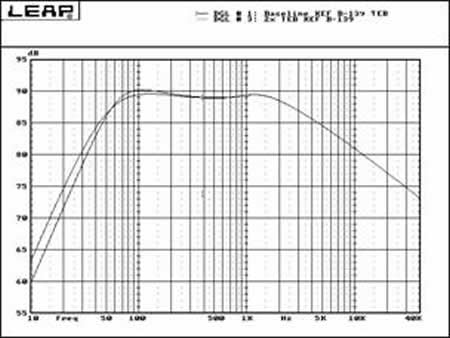
Figure 16: Response plots for Baseline TEB and 2xVB TEB
I started with a comparison of the baseline system to a system where Vb was doubled, with all other design parameters held constant. This doubling of the net internal cabinet volume used for the baseline design did very little to change overall response and nothing in the passband reference efficiency region as shown by the supporting graphic. (As you read through the graph data, keep in mind that each vertical dB SPL axis is scaled in 1dB units).
BaseLine AUC: 3138748 2xTEB AUC: 3138695 | Δ | = .001%
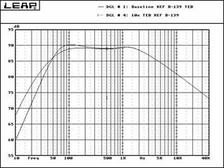
Figure 17: Response plots for Baseline TEB and 10x VB TEB
I then re-ran the simulation, this time modeling a system with a net internal cabinet volume 10 times larger than that of the baseline system. Even with a one order of magnitude increase in net Vb, we observe no change in η0dB of the system; it still hovers extremely to that of the driver.
BaseLine AUC: 3138748 10xTEB AUC: 3138627 | Δ | = .0038%
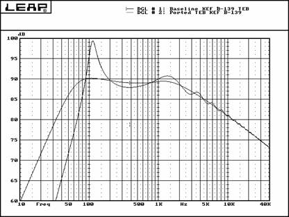 Next, I took the baseline TEB system and, virtually, cut a port in the cabinet. The port modeled had a .75" depth, and a cross-sectional area of .5 * Sd (.017545). All other parameters were, as before, held constant. I then re-ran the simulation, producing the result we see here.
There are in this graph some noteworthy items. First, we see the mid-band reference efficiency of the ported system has actually dropped , while at the same time a ~ +10dB local maximum has appeared at just a bit above 100 Hz.
I've Included beneath each graph an
area under curve (AUC) value generated by performing an integration on the response plot from 10 Hz to 40kHz. The | Δ| value represents the absolute value of the % difference found when comparing the AUC value of the baseline TEB vs each of the other 4 systems modeled. I included the AUC as had there been any substantial differences in the resulting simulation η0dB values; it would have shown up as a |Δ| far larger than the vanishingly small values which we see here.
Figure 18: Response plots for Baseline TEB and Ported TEB
BaseLine AUC: 3138748 Ported TEB AUC: 3138952 |Δ| = .006%
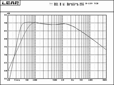 Last, I compared the baseline TEB response with that of a BR system, featuring, as in each preceding case, the test driver specced above. Here we observe the bandwidth extension which we would expect for a properly designed & tuned BR cabinet. Once again, there is no change evident in the observed pass-band η0dB value.
From these graphs we can conclude that simply cutting a hole in a TEB cabinet or increasing the size of the cabinet will not increase η0dB values. We've also seen that, in some cases, such modifications can decrease system η0dB.
We've also observed one can design a TEB and BR system with the same driver and come up with a BR system that sports an extended LF response when compared with that of the TEB, but that won't change the η0dB value either, as the graphs clearly indicate. An increase in bandwidth - yes, but a change in reference efficiency - no.
Figure 19: Response plots for Baseline TEB and BR system.
BaseLine AUC: 3138748 BRKEF AUC: 3139468 | Δ | = .0229%
To understand why for each of the systems modeled the η0dB values determinedly remained within a small fraction of a dB of the test driver's reference efficiency value, let's take a look at the mathematical underpinnings of driver & system efficiency. We'll also see why system η0dB hovers near or below driver η0dB but never exceeds the driver's η0dB value.
From:

we can calculate a driver's reference efficiency.
Where:
η0 = reference efficiency of the driver, dimensionless
ρ0 = the density of air at STP, 1.204 kg/m^3 @ 20?C
c = speed of sound at STP, 343.4 m/s @ 20?C
B = magnetic flux density in the driver air gap, in Tesla
l = length of the voice coil winding in the gap, m
Revc = DC resistance of the driver voice coil, Ohms
Mms = mechanical mass of the driver diaphragm assembly, including air load, Kg
Sd = effective projected surface area of the driver diaphragm, m^2
From:

we can calculate the reference efficiency of a closed box system where:
η0 = reference efficiency of the system, dimensionless
kη = efficiency constant, dependent upon chosen alignment,  , given by:
kη = 
fc = closed box system resonant frequency
f3 = -3dB cutoff frequency of the system
c = speed of sound at STP, 343.4 m/s @ 20?C
Qec = System electrical Q at fc
Vb = net internal volume of enclosure
Vat = total system compliance expressed as equivalent volume of air, l
For closed box systems, kη maxes out at ~  .
.
This figure represents a maximum performance limit and can be reached only by employing a lossless system, based on the C2 alignment.
For vented systems we have, once again:
where:
η0 = reference efficiency of the system, dimensionless
kη = efficiency constant, dependent upon chosen alignment, , given by:

fs = driver resonant frequency
f3 = -3dB cutoff frequency of the system
c = speed of sound at STP, 343.4 m/s @ 20?C
Qes = driver electrical Q at fs
Vas = volume of air having same acoustic compliance as driver suspension
Vb = net internal volume of enclosure
For vented systems, kη maxes out at ~  . This figure represents a max performance limit and can be attained only by employing a lossless vented system, based on a k = .5, C4 alignment.
In all three cases, η0 values can be converted to power sensitivity in decibels by:
η0dB = 112.2 + 10 * Log (η0) (dB SPL/1W/1m)
or, alternately, converted to percent by:
η0% = 100 * η0 (%)
Efficiency, broadly defined in this context, is the ratio of acoustic power out to electric power in:

Where both PA and PE are in watts.
The two system reference efficiency equations tell us that enclosure volume, cutoff frequency and maximum reference efficiency are interdependent. Small refers to this as the "Efficiency-Bandwidth-Volume Exchange". Given the alignment type and losses present, η0 can be maintained while altering either f3 or Vb only by altering the value of the remaining factor. Want a lower f3? You'll need to increase Vb. Want a smaller cabinet? You can expect f3 to rise, presuming, of course, that you want to maintain a particular η0 - or ratio of acoustic power out to electric power in - value constant.
Keep in mind that the calculated system η0 values represent an ideal performance maximum: the best you could hope for, given a specific alignment resulting from a specific design for a specific driver. In practice, actual system η0 values are lowered or constrained by such things as driver mechanical losses, enclosure losses and employing alignments other than those mentioned previously as being maximally efficient. Therefore, it's not difficult - by choice or chance - to design a system that exhibits a lesser actual η0 value. Loudspeaker design is a study in artful compromises; what you trade away in one area to gain in another depends upon, among other things, what your design priorities and goals are. If, in this case, for a given driver every design permutation you model delivers insufficient η0dB values, the only to increase the values would be to switch to a more efficient driver.
Above resonance, but below fh, the driver is operating in its inertial mass-controlled reference efficiency passband. As such, in this portion of its output spectrum, the cone is mass-limited and the driver functions as a constant acceleration device, producing constant volume velocity. An enclosure does not change the mass of the driver cone, so it cannot affect efficiency as constrained/controlled by cone mass. The air within the cabinet does not provide resistance to the motion of the cone; if it did varying cabinet size would produce varying observed η0dB levels. We do not observe such variations across the 5 simulations (even in the case where cabinet size is increased by a factor of 10). Given that a driver's reference efficiency is taken from the mass-controlled region of its response, a driver's efficiency is independent of an enclosure's volume, whether said enclosure is vented or not. Neither does an enclosure alter a driver's Bl , Sd or Mms.
So essentially we see no real variations in η0dB levels across each of the 5 simulations because the cabinet does not affect or otherwise alter the driver parameters that determine its reference efficiency. Hence we never see a system sporting η0dB levels greater than that of the driver, but given a variety of factors we can see a cabinet/driver combination that lowers η0dB levels that could otherwise be attained.
5. The Perfect Driver....
… would be infinitely stiff and completely massless.
I think this myth has survived as long as it has because, at first glance, the assertion seems to make sense; after all a driver that is infinitely stiff and has no mass should have zero problem responding perfectly and instantly to every electrical impulse fed it's inputs, right? Let's see what a bit of examination behind the scenes of the typical bandpass response of moving coil driver turns up.
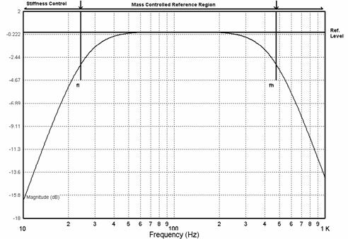
We can divide the response curve roughly into 3 regions, each demarcated by, fl, lower resonance and, fh, upper resonance. (Would that all drivers had such well-behaved response curves!)
Below fl, stiffness (or its inverse, compliance - as supplied by the driver's suspension - expressed as Cms) predominates in limiting the motion of the cone and output is proportional to frequency ^ 4. Which, below resonance, means a roll off of 12dB/octave as frequency drops. In this region the driver functions as a constant excursion device.
At fl, output depends on resistance, including Rsource and Revc. The frequency at which fl occurs is determined by the moving mass of the driver. And as the theoretical moving mass of our driver → 0, fl approaches ∞ Hz. As shown by:
fs = .5π * (1/(Cms * Mms))^.5 (Hz)
Where:
fs = Free air resonance of driver, Hz
Cms = Mechanical compliance of driver, m/N
Mms = Effective mechanical mass of driver diaphragm, in kg
Between fl and fh is the mass-controlled reference region of the driver. In this portion of its output spectrum, the cone is mass-limited and the driver functions as a constant acceleration device, producing constant volume velocity. Radiation remains essentially hemispherical and directivity, constant.
At fh, like fl, resistance plays the controlling role. Fh can be determined by:
fh = ω*Levc*B^2l^2
--------------------------------------
ω^2*Levc^2 + (Rg + Revc)^2
and total resistance at fh can be found by:
Rtotal = (Rg + Revc) * B^2l^2
------------------------------------10
(Rg + Rc)^2 + ω^2* Levc^2
Figure 20: Bandpass response of a generic electromagnetic driver
So where's the problem with the infinitely stiff/massless driver?
By setting stiffness to ∞, fl is pushed up to ∞ Hz (besides sounding painful in an abstract sort of way), means that since response rolls off at 12/dB per octave, by the time frequency has dropped to within the audible range response is -∞ dB down, hence no output.
Above fl = ∞, our incredible driver is, predictably, functioning as a constant acceleration device generating a flat frequency response, but as its all happening at a frequency of ∞ Hz, there's no audible output. Our perfect driver remains, as far as human hearing goes, silent. There exists a whole host of other technical issues that would contribute to the driver's zero output (e.g. out of phase cancellation), but just focusing on Cms = 1/∞ and Mms = 0 are, in and of themselves, sufficient to silence the myth.
Ferreting out the facts behind a myth - or any facet of loudspeaker design, for that matter - can be enjoyable, satisfying and enlightening. Like a detective story where every clue is important, you can find yourself developing an almost child-like curiosity when investigating the facts using whichever tool you have at hand: mathematics, CAD, your calculator or a workbench with a bunch of analog test gear on it. The Internet, while providing forums for the propagation of audio myths is also a formidable tool in providing many resources useful to sorting the facts from fiction. Perhaps the greatest benefit of all such research is that, in the end, you can only gain in understanding. In this article I've shared what I've uncovered in the course of my examinations and would hope you too have gained in your understanding by reading it.
Resources
Ashley, Robert j. and Saponas, Thomas A, Wisdom and Witchcraft of Old Wives' Tales about Woofer Baffles , Journal of the Audio Engineering Society, Vol 18, November 5, October 1970
Benson, J. E., Theory & Design Of Loudspeaker Enclosures, Howard W. Sams & Company, Indianapolis , IN., 1996
Colloms, Martin, High Performance Loudspeakers, John Wiley & Sons, 1978, New York
D'Appolito, Joseph, Testing Loudspeakers, Audio Amateur Press, Peterborough, New Hampshire, USA, 1998
Dickason, Vance, The Loudspeaker Design Cookbook, 5th Edition, Audio Amateur Press, Peterborough, New Hampshire, USA , 1998
Faucett, Max A., Kraehenbuehl, John O., Circuits And Machines In Electrical Engineering , John Wiley & Sons, New York, 1939
Greiner, R. A., Amplifier-Loudspeaker Interfacing, Journal of the Audio Engineering Society, Vol. 44, Number 12, December 1996
Griffiths, David J. Introduction To Electrodynamics, 2nd Edition, Prentice Hall, Englewood Cliffs, NJ USA 1989
Harrison, Jeffrey, An Integral Limitation upon Loudspeaker Frequency Response for a Given Enclosure Volume , Journal of the Audio Engineering Society, Vol. 44, Number 12, December 1996
King, John, Loudspeaker Voice Coils, Journal of the Audio Engineering Society, Vol. 18, Number 1, February 1970
Locanthi, Bart, Application of Electric Circuit Analogies to Loudspeaker Design Problems, Journal of the Audio Engineering Society, Vol. 19, Number 9, October 1971
Magnetic Shielding Lab Kit With AC Probe, Brochure, Magnetic Shield Corp, Bensenville , Illinois , USA
Novak, James F., Performance of Enclosures for Low Resonance High Compliance Loudspeakers, Journal of the Audio Engineering Society, Vol. ??, Number ?, January 1959
Sanfilipo, Mark, Inductor Coil Crosstalk, Speaker Builder
Small, Richard H., Closed-Box Loudspeaker Systems Part I: Analysis , Journal of the Audio Engineering Society, Vol. 20, Number 10, December 1972
Small, Richard H., Closed-Box Loudspeaker Systems Part II: Synthesis , Journal of the Audio Engineering Society, Vol. 21, Number 1, Jan. /Feb. 1973
Small, Richard H., Direct-Radiator Loudspeaker System Analysis , Journal of the Audio Engineering Society, Vol. 20, Number 5, June, 1972
Small, Richard H., Vented-Box Loudspeaker System Part l: Small-Signal Analysis , Journal of the Audio Engineering Society, Vol. 21, Number 5, June, 1973
Small, Richard H., Vented-Box Loudspeaker System Part ll: Large-Signal Analysis , Journal of the Audio Engineering Society, Vol. 21, Number 6, July/August, 1973
Thiele, A. N., Loudspeakers in Vented Boxes: Part l , Journal of the Audio Engineering Society, Vol. 19, Number 5, May, 1971
Thiele, A. N., Loudspeakers in Vented Boxes: Part ll , Journal of the Audio Engineering Society, Vol. 19, Number 6, June, 1971
Weidner, Richard T., Physics Allyn & Bacon, Inc, Needham Heights, MA, 1989
Yarbrough, Raymond B., Electrical Engineering Reference Manual , 5th Edition, Professional Publications, Belmont, CA, 1990