
Subwoofer Measurement Tactics: A Brief, Topical Overview & Method Comparison
Axiom Sub
The challenges of accurately capturing the direct sound amplitude response of a subwoofer, especially for the enthusiast who would not likely have access to the facilities or hardware typically available to the professional, are well known and widely discussed in print and online.
In this brief overview, we’ll take a look at a variety of measurement approaches that when correctly implemented can minimize or in some cases altogether eliminate the complicating influence of room\boundary\subwoofer interaction. The scope of this overview is limited to subwoofers only and the amplitude response frequencies range of 10 Hz to 320 Hz.
This is by no means a detailed treatise of the subject. For a more in-depth treatment of this topic the reader is encouraged to read through the resources listed in the bibliography.
|
Measurement Approach/Domain Space |
Implementation |
Advantages |
Disadvantages |
Limits |
|
Anechoic Chamber |
Acoustical measurements done within an indoor, (ideally) reflection-free environment |
Climate-controlled, artificial environment in which to measure amplitude response, noise & distortion, diffraction effect & directional response characteristics |
Cost; extremely large chamber needed for accurate LF amplitude response, noise & distortion, etc measurement |
Chamber , device under test (DUT) size; depth, type & configuration of absorptive material used within the chamber |
|
Tower/Crane Measurement |
Acoustical measurement done out of doors, with DUT mounted on a tower or suspended by crane |
Under appropriate conditions, can provide for an ideal free-field measurement environment |
Cost, Requires DUT be placed well away from any reflective surfaces or objects large enough to influence measurements |
Noise pollution, inclement weather |
|
Ground Plane Measurement |
Measurement done with the DUT & microphone typically placed on the ground, with the emissive radiating surface(s) pointed at the microphone |
Low cost; ease of implementation, within known limits, can provide accurate measurement data |
Upper & lower frequency limits. Other than the ground upon which it rests, DUT must be placed well away from any reflective surfaces or objects large enough to influence measured amplitude response |
Noise pollution, Inclement weather (when done outdoors) |
|
Half-Space or Hemispherical Free Field Measurement |
Device affixed flush-mount with surface such as baffle, ground surface or clear wall of Hemi-anechoic chamber |
Depending on implementation and type of data sought, can provide excellent results |
Cost of indoor Hemi-anechoic chamber; use of baffle invites cancellation?. Out door, in-ground placement requires DUT to be placed well away from any reflective surfaces or objects large enough to influence measurements |
Approach requires all emissive radiators be on one side of the cabinet |
|
Windowing |
Measurement taken and unwanted data windowed out |
Fast data acquisition & post-processing |
Requires significant data post-processing and the ability to skillfully interpret the results |
LF measurement accuracy defined by environmentally determined window length. Poor tolerance for time variance. |
|
Near Field Measurement |
Measurement done with microphone placed near to, centered on and normal to front emissive surface of each acoustic radiator |
When implemented correctly, the near-field amplitude response provides for an accurate facsimile of the far field response |
Multiple emissive surfaces require multiple measurements along with subsequent post processing |
Upper frequency limit determined by size of DUT. |
I. Anechoic Chamber
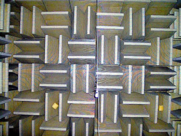
An anechoic chamber, in the literal sense, is a “chamber without echo”. Generally speaking, a chamber is commonly considered anechoic at any particular frequency when 1% (or less) of the acoustic energy impinging on the absorptive material lining the walls of the chamber is returned to the clear space or “lumen” of the chamber. The idea here is to create a free-field acoustic environment in which to assess a variety of loudspeaker acoustical performance characteristics such as amplitude response, directionality, distortion and so forth.
The necessary free-field conditions occur when the sub appears as a singular or sole point source, radiating spherically (4π sr) into an anechoic environment. (The sub behaves as a point source when the wavelength, λ, of the sound radiated is >> than its largest dimension). The measurement mic is then positioned far enough away from the sub so that it is within that portion of the sub’s sound field where the sound pressure level drops -6dB for every doubling of distance. The mic would now be considered in the sub’s Far Field.
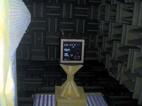
Being accustomed as we are to the ever-present noise of everyday life, stepping into the reflection-free silence of an anechoic chamber can be an odd, vaguely disorienting experience. Paradoxically, its precisely those characteristics that give rise to this odd sensory experience of that very artificial environment which make it ideal for the purpose of capturing accurate data needed to correctly assess various acoustical performance characteristics of a subwoofer.
Though there are certainly challenges to be found in designing a chamber to perform anechoically in the mid- and high-frequency portions of the audible spectrum, it’s the low frequency portion of the audible spectrum where practical limitations come into play and the design process becomes especially challenging. When the 1% reflected acoustic energy figure cited above is reached, that’s typically considered the useful (ie anechoic) LF limit of the chamber being assessed.
These LF performance limitations are defined by a number of factors, including the overall linear dimensions and enclosed volume of the chamber, the depth/distributed density of the absorptive wedges populating the interior surfaces of the chamber, (along with the mechanical/acoustical properties of the wedges themselves) and the size of the DUT. A chamber useful for measurements down to ~ 30 Hz would require an internal volume of over 4700 m^3 (166k ft^3) and sport wedges over ~3m (9.8 ft) in depth.
The basic principal behind the typical anechoic chamber design is that of a collection of boundaries, functioning as purely resistive acoustic loads, absorbing progressive plane waves. The assumption made here is that the absorptive surfaces are hit by the waves, which themselves sport a specific acoustic impedance, Z, which is purely real. This assumption holds true if the distance from the source (namely, your subwoofer) generating the spherically diverging waves to the absorptive wedges is sufficient in distance so as to present, for all intents and purposes, progressive plane waves to the boundaries. This assumption does not necessarily hold true at low frequencies, hence the LF limits.
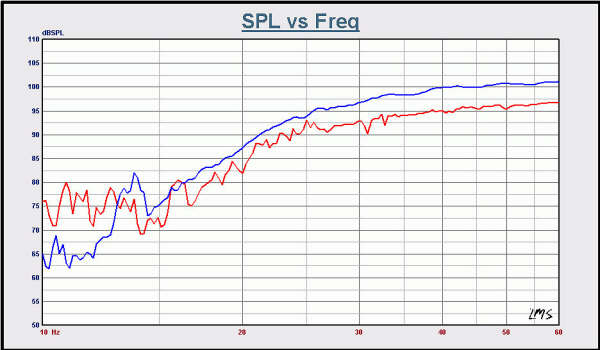
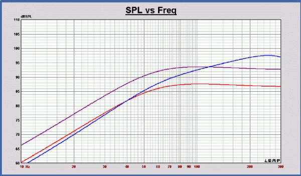
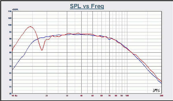 At right are
two amplitude response plots of the same sub. The blue is that of the sub
measured outdoors, on a tower and raised 100’ in the air. The red plot is that
of the same sub, now measured in an anechoic chamber. The anechoic chamber’s
ability to absorb & dissipate acoustic energy in the < 30 Hz band
progressively diminishes as the measurement frequency approaches 10 Hz. The
chambers absorptive ability’s have clearly been exceeded.
At right are
two amplitude response plots of the same sub. The blue is that of the sub
measured outdoors, on a tower and raised 100’ in the air. The red plot is that
of the same sub, now measured in an anechoic chamber. The anechoic chamber’s
ability to absorb & dissipate acoustic energy in the < 30 Hz band
progressively diminishes as the measurement frequency approaches 10 Hz. The
chambers absorptive ability’s have clearly been exceeded.
Increasing the linear dimensions of the chamber and the depth/density (that is to say the resistive/reactive characteristics) of the absorptive wedges is one way to extend the LF limit of a chamber. An alternative, typically less costly approach, is constructing absorptive surfaces such that they present a reactive boundary at low frequencies and a resistive boundary at mid- and high-frequencies. Referred to as an “acoustic jungle”, the absorptive arrays, rather than the usual wedges, comprise arrays of absorptive blocks, differing in size & density, built up in a way such as to present just such a reactive/resistive boundary surface.
Practically speaking, making use of an anechoic chamber to measure your sub can present a variety of possibly insurmountable challenges to the audio enthusiast: rental cost, lack of access, extremely low SAF if you build one (unless you own the company). Nevertheless, from a strictly scientific or engineering standpoint, anechoic chambers remain an ideal, indoor measurement environment.
II. Outdoor (Tower/Crane) Measurement
For the pro & audio enthusiast alike, outdoor measurement is an attractive alternative. At its best, it can provide for a measurement environment that rivals (or in some cases) surpasses that of an anechoic chamber. The downside, of course, in taking your subwoofer & measurement gear outdoors is that you now have the weather as well as background noise pollution to contend with.
But let’s suppose for a moment the weather is cooperating and the background noise pollution is minimal or otherwise of a nature that a dose of curve-averaging can properly deal with. How then to attain at or near anechoic measurement conditions?
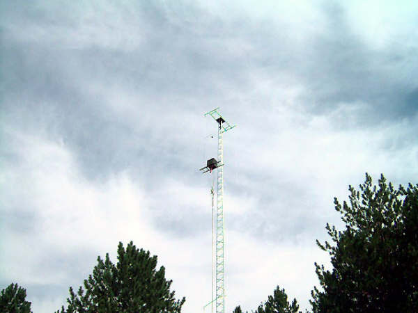
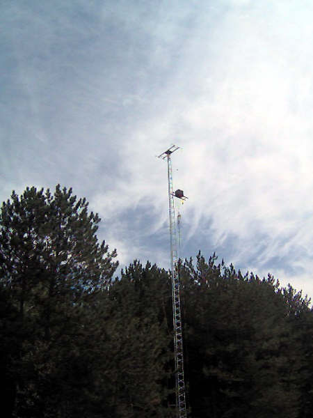
One method is to mount the sub on a stand, pole, tower, boom placed well above the ground or haul it up with a crane. There are, of course, always practical constraints (as well as safety issues) involved where it comes to just how high above the ground you can place the sub. Strictly from a measurement perspective, though, the higher the better.
The idea here is to get the sub as far away from any
response-muddling reflective boundaries as possible. Given the wavelengths
involved (a 20 Hz wave is approximately 17 meters (56.5 feet) long) it can be
quite challenging, if not altogether impossible,
to get the sub as high above the ground as you might like. Nevertheless, get
the sub high enough and you will be measuring in an ideal anechoic, free field
environment. Indeed, data taken under such conditions can be clean & accurate
enough that you can build mic correction files with it. Because the quality of
measurement data taken under the aforementioned conditions is so good, the
baseline amplitude response used for comparison purposes in this article will
be that of the test sub measured at the top of the tower. This correction file could be used to develop an accurate low frequency response measurement in an anechoic chamber.
If you don’t own or otherwise have access to a 100’ tower, like that showing in Figs. 3a & b above, or any other means by which to remove the sub from the vicinity of any reflective surface, no need to worry; there are still other approaches that can be used that in practice cost little or nothing.
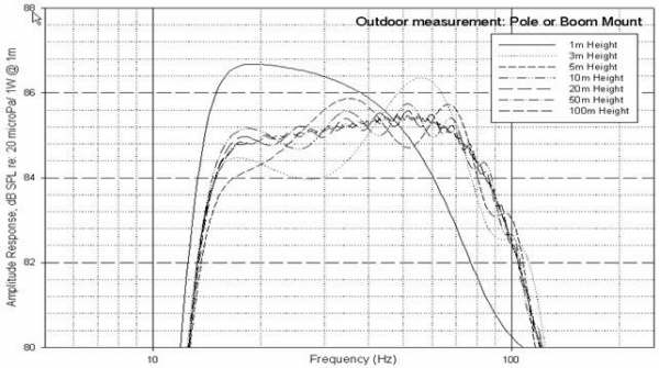
Plot 1: Akabak Model: 12” Driver in totally enclosed box. Note how curves progressively flatten as height is increased.
The next best alternative to measuring a subwoofer on a pole would be to place it on the ground. This measurement is known as the "Groundplane technique" which is our next topic of discussion.
Subwoofer Measurement Tactics: Methods Continued Page 2
III. Ground Plane Measurement
We now come to an option that doesn’t require much more than a flat, solid, unobstructed surface such as an asphalt or concrete driveway or parking lot to rest the sub and measurement microphone on. Obviously, in being outdoors, you’ll once again be at the mercy of the elements as well as background noise pollution.
Don’t underestimate the latter’s measurement-corrupting capabilities: air or ground traffic or wind noise can easily mangle an otherwise good amplitude response measurement, as evident in the < 15 Hz portion of the blue and < 25 Hz portion of the red curves seen above . Depending on the nature of the background noise, redoing the measurements when all is quiet or averaging several measurements are effective antidotes.
Where the tower approach represents an attempt to eliminate boundary reflection by placing the sub well away from any reflective surfaces, ground plane measurement takes into account the effect of the single boundary the sub sits on. The acoustic signal reflected from the ground surface is considered to be a second, virtual source, identical to the actual source.
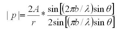
Based on the well proven, time tested method of images, ground plane measurement is an approach solidly grounded in science. To see why it works as well as it does, let’s look at the equation for the magnitude of the rms sound pressure, |p|:
 (1)
(1)
Where:
|p| = magnitude of the rms sound pressure
A = magnitude of the rms sound pressure at unit distance from the center of each source
r = measurement distance
b = distance between the center of actual and virtual acoustic image
λ = wavelength of frequency under consideration
θ = angle to the perpendicular bisecting the actual and virtual acoustic images
Note that eq. 1 is for 2 acoustical sources, in this case the sub’s actual and virtual acoustic images.
At low frequencies (ie long wavelengths, where λ >> b), b is relatively small by comparison and the actual & virtual source will appear as a single source with sound pressure double that of the actual source alone. This doubling results in a 6dB increase of the measured axial sound pressure level above that produced by the same sub measured at the same distance under perfectly anechoic, free field conditions.
Care must be taken to ensure that measurements are, ideally, made with no large objects or reflective surfaces (other than the ground the sub sits on) within a radius ≥ λLF/2, where λLF equals the wavelength of the lowest frequency of interest. In this case a large “object” might be a barn or your neighbor’s house; a large reflective surface might be, for example, the side of a nearby apartment building or office tower.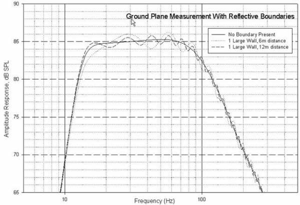
Plot 2: Akabak Model: 12” Driver in totally enclosed box. Note interference effects from nearby boundaries.
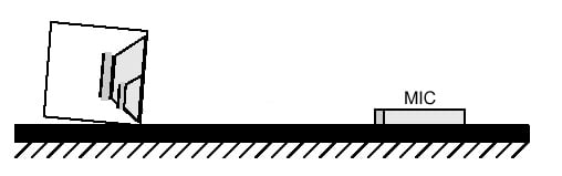
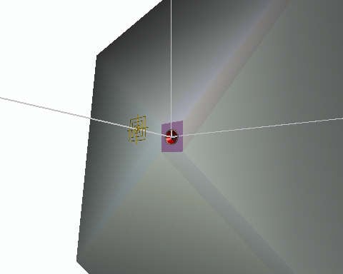
Setting up for a ground plane measurement is pretty straightforward. Position the sub so its driver(s) are facing the measurement microphone; that is to say, lay the thing on its side. Then tilt the cabinet until the center axis, normal to the driver (or panel into which the drivers have been bolted, if 2 or more drivers are used) points to a spot on the ground 2 meters away. You may find using a laser pointer handy. Once the subwoofer has been oriented correctly, place the measurement microphone at the exact spot where the axis intersects the ground and measure away. But why measure at 2 meters when amplitude response measurements are typically made at 1 meter?
When the virtual & actual acoustic image outputs combine at the microphone, the net effect is to add 6dB to the axial sound pressure level. Doubling the measurement distance from 1 meter to 2 meters decreases the axial sound pressure level by 6 dB. As mentioned above, do so and the net result at the frequencies of interest produced by the subwoofer, is that the response will very nearly mirror that of the subwoofer measured free-field (or in an ideal anechoic chamber) only slightly altered by a few unavoidable acoustical artifacts.
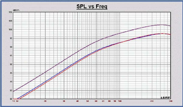
Working up a model (15” driver in totally enclosed box) in LEAP 5 (plots at right), we see the reference free-air curve in blue, ground plane @ 1 m in purple and the ground plane curve scaled to 2m (red). As expected, the ground-plane at 2m is nearly identical to the free-air plot at 1m. Clearly, the ground-plane approach is an excellent, cost-effective (if not outright free) alternative if you don’t happen to have handy an anechoic chamber or a 100’ tower.
Given the ease of implementation, the data quality typically attainable and the minimal post-processing requirements, the ground-plane measurement technique (when done outdoors) is likely the best options available to the audio enthusiast.
Subwoofer Measurement Tactics: Methods Continued Page 3
IV. Half-Space or Hemispherical Free Field Measurement
This approach places either a raw driver or the front panel of the loudspeaker system within and flush with a large baffle. The rationale often cited for making use of this approach is that in changing the domain space from 4π steradian (spherical) to 2π steradian (hemispherical) the resulting amplitude response measurements will more accurately portray the low frequency performance of the system within a typical listening environment.
In practice, the usual implementations of this approach make use of either a simple, large baffle, (as per IEC standard 268 -14) for driver testing, a hemi-anechoic chamber or simply burying the system in the ground (or other large flat surface, such as a roof) with the driver or the faceplate of a complete system positioned upward and flush with the test surface.
From a practical standpoint, digging a hole in the backyard to measure your sub’s amplitude response isn’t typically found in the list of items guaranteed to result in a positive SAF. Besides all that, what if your sub is a vented system with the ducts firing out any panel other than the one the driver(s) are bolted into - how are you going to bury that?
Modeling again in LEAP 5, the plots showing at above left are free-air (blue), half-space @ 2m (red) and half-space @ 1m (purple).
V. Time-Windowed Impulse/MLS
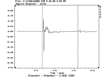
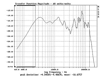
The time-windowed measurement approach has a number of immediately attractive qualities that have made it a popular tool when it comes time to assessing various acoustical performance characteristics of a loudspeaker. Essentially, it works as follows: an impulse or Maximum Length Sequence signal (MLS: a deterministic signal with spectral properties similar to that of white noise) is first applied to a sub and the measured response is then run through a variety of post-processing utilities (See figure, above, Left), in turn producing ETC curves, frequency response plots, cumulative spectral decay (aka waterfall) plots and so forth (See figure, above, right).
Probably the most intuitively appealing feature of this particular approach is the option to window out all but the anechoic portion of the measured acoustical signal. Sounds ideal for subwoofer measurement, doesn’t it? However, in practice this approach is limited in terms of how accurate the LF results can be by, among other things, the prevailing acoustical/environmental conditions.
Suppose for a moment you’re measuring your sub’s performance indoors and owing to reflections you find you need to window out all data beyond 10ms. Within that time window, the largest complete sinusoidal period that can be completely contained is 10 ms long. Any data featuring wavelengths possessing a longer period than that (i.e. anything lower in frequency than 1/10ms = 100 Hz) will be inaccurately presented, more so the lower the frequency. Any inaccuracy existing in the initial, raw measurement data will of course carry through to whatever results are generated through post processing.
As dreary as this might sound to anyone contemplating using
this approach in measuring a sub, there are workarounds that allow for accurate
time-windowed measurements - even under less than ideal circumstances - such as
preprocessing the test signal, measuring with a mic specifically calibrated for
the environment/set up your using or making time-windowed
measurements in the near-field, a topic
covered in the next section.
VI. Near Field Measurement
The near field approach, when done correctly is a simple, yet very effective means for capturing the direct sound amplitude response of your subwoofer. Where it comes to measuring subs, many of the practical limits or issues faced when employing some of the alternate approaches illustrated above are simply rendered moot at the frequencies of interest. If your only option is to measure your subwoofer indoors, this is probably the best – and easiest - approach to take.
 From Eq 2:
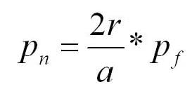 (2)
(2)Where:
pn = peak pressure in the near field at the center of the piston (driver diaphragm)
r = distance from measuring point (mic position) to the center of the piston
a = piston radius
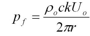 , peak axial pressure measured at a distance, r, in the far
field of the piston
, peak axial pressure measured at a distance, r, in the far
field of the piston
ρo = density of air, = 1.21 kg/m3 at 20° C
U0 = piston peak output volume velocity
k = wave number, = 2π/λ = ω/c
c= velocity of sound in air, = 343 m/s
We see that for those frequencies of interest (ka < 1), the near field sound pressure is directly proportional to far field sound pressure and the measurements made in the near field are basically independent of the space into which your subwoofer is firing; measuring “near” and scaling to “far” is valid & accurate. The upper frequency boundary for accurate near-field measurements is reached when a/λ ~ .26
In addition to being an effective means by which to measure a sub’s amplitude response, this technique (when done correctly) also allows for equally valid measurements of system distortion, efficiency and total acoustic power. It can be used to measure either closed or vented systems, powered or passive.
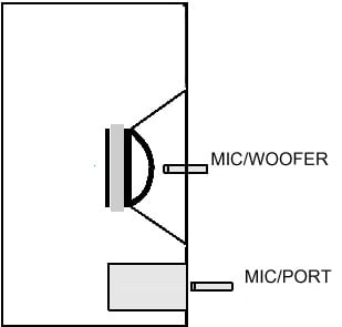
The near-field sound pressure measurement technique requires the measurement microphone be placed in a position centered on and normal to the driver’s dustcap and no further away from the center of the radiator than .11a (r ≤ .11a), assuming measurement data accurate to within 1dB or less is the goal. If you’re measuring a vented system, you’ll need to measure separately the acoustic output of the driver(s) and port(s). When measuring the latter, you’ll need to place the mic centered on & normal to the duct’s port, flush with the system’s faceplate.
Where there is only one radiator, such as a sub comprising a single radiator (driver) in a totally enclosed box, you need only measure the driver’s near-field output and scale the resulting data. If you’re measuring a vented system (or any system featuring more than one radiator, be it port(s), driver(s) or passive radiator(s)), then individual measurements are made of each radiator and the data are then combined to produce the total system amplitude response. Because all measurements are being taken near-field, the data should be scaled to an appropriate distance, commonly 1 or 2 meters. So how do you scale the nearfield measurement data to, say, 1m? To calculate the near-field scaling factor (1m, half-space) use:
FFdB = NFdB - 20 * Log(0.2821 * SQRT(Sd)) (dB) (3)
Where: Sd is the effective diameter of the radiator, m^2
(To calculate the 1m, full-space (anechoic), far-field equivalent, use the above equation and
subtract 6dB from the results).
Here are some alternate equations useful in scaling NF to FF measurement data:
FFdB = NFdB - 20 * Log(4d/r) dB, 4π-space (4a)
and
FFdB = NFdB - 20 * Log(2d/r) dB, 2π-space (4b)
Where:
FFdB = scaled far-field dB value
NFdB = near-field dB value
d = distance at which far-field values are to be calculated (eg: 1m)
r = effective radius of radiator
Note: units (m, in, cm, etc) must be the same for both d & r
Refer to the chart below for the Sd values for a variety of nominal driver sizes:
|
Nominal Driver Size (Diameter) Sd (m^2) |
Sd (m^2) |
|
24 Inch (610 mm) |
0.2200 |
|
18 Inch (460 mm) |
0.1300 |
|
15 Inch (380 mm) |
0.0890 |
|
12 Inch (300 mm) |
0.0530 |
|
10 Inch (250 mm) |
0.0330 |
|
8 Inch (200 mm) |
0.0220 |
|
6½ Inch (170 mm) |
0.0165 |
|
6 Inch (150 mm) |
0.0125 |
|
5¼ Inch (140 mm) |
0.0089 |
|
4½ Inch (110 mm) |
0.0055 |
|
3 Inch (80 mm) |
0.0038 |
Should the distance between driver(s) and port(s) be significant in terms of the wavelengths of interest, the maths become a bit more complex if data of the highest quality is your requirement. Neville Thiele wrote a concise paper on the maths involved, referred to in the bibliography.
Before commencing any near-field measurements, be certain your measurement mic can handle the acoustic output dished out by the radiator(s) at close proximity. This holds especially true if you’re interested in doing max. dB spl output testing.
Also, when setting drive levels its best to do a number of test runs, working up each time to determine driver excursion so you don’t end up with the mic getting hit by the unit’s diaphragm when doing the actual measurements. As well, to ensure accurate port data, avoid using drive levels so high as to introduce turbulence in the port.
Conclusion
In this brief overview we’ve looked at a variety of approaches to subwoofer measurement. Each has its own set of strengths, weaknesses and limitations. Success in capturing accurate data depends on correctly understanding how to measure, how to interpret the results and above all remaining cognizant of the limitations inherent to whichever approach is used. And if all else fails, there’s not much a little 1/3rd-octave smoothing won’t make look good.
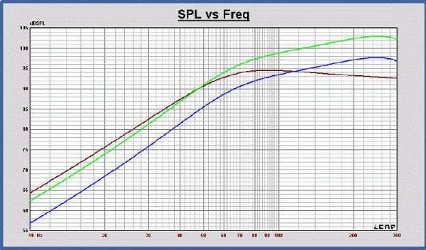
As a handy reference, a graph featuring plots of a system modeled in the half-space, ground plane and free-air space domains, along with an accompanying table are included below.
|
|
Relative Gain @ 1m, Drv. Level Held Constant |
Comments |
|
Free-space |
0 dB (reference) |
Half-space & Ground Plane amplitude response plots referred to this plot |
|
Infinite Baffle |
~+6dB @ low frequencies |
Gain relative to free-space amplitude response varies with frequency. Diffraction plays no roll in determining amplitude response. |
|
Ground Plane (green trace) |
+6dB |
Holding drive voltage constant, but measuring @ 2m gives results virtually identical to those obtained measuring Free-space |
Resources
1. Allison, R. F. and Berkovitz, R.: “The Sound Field in Home Listening Rooms” Journal of the Audio Engineering Society, Vol. 20, July/Aug. 1972
2. Benson, J E., “Theory & Design of Loudspeaker Enclosures”, Howard W. Sams & Co., Indianapolis, IN, 1996
3. Berman, J. M. & Fincham, L. R.: “The Application of Digital Techniques to the Measurement of Loudspeakers” Journal of the Audio Engineering Society, Vol. 25, June 1977
4. Bjor, Ole H.: “Maximum Length Sequence” Norsonic AS, 2000
5. Brüel, Dr. Per V., “Anechoic Chambers”, Technical Review 96-02, Brüel Acoustics, 1996
6. D’Appolito, J.: “Testing Loudspeakers”, Audio Amateur Press, Peterborough, NH, 1998
7. Dunn, Chris & Hawksford, Malcolm., “Distortion Immunity of MLS-Derived Impulse Response Measurements”, Journal of the Audio Engineering Society, Vol. 41, #5, May 1993
8. Fincham, L. R.:, “Refinements in the Impulse Testing of Loudspeakers”, Journal of the Audio Engineering Society, Vol. 33, #3, October 1983
9. Fincham, L. R.:, “Production Testing of Loudspeakers Using Digital Techniques”, Journal of the Audio Engineering Society, Vol. 27, #12, December 1979
10. Gander, Mark R., “Ground-Plane Acoustic Measurement of Loudspeaker Systems”, Journal of the Audio Engineering Society, Vol. 30, #10, October 1982
11. Geddes, Earl R., “On Sound Radiation from Ported Enclosures”, Journal of the Audio Engineering Society, Vol. 49, #3, March 2001
12. Griesinger, David.: “Beyond MLS - Occupied hall measurement with FFT techniques ” Lexicon, Waltham, MA
13. Keele, Don B., “Anechoic Chamber Walls: Should They Be Resistive or Reactive at Low Frequencies”, Journal of the Audio Engineering Society, Vol. 42, #6, June 1994
14. Keele, Don B., “Low-Frequency Loudspeaker Assessment by Nearfield Sound-Pressure Measurement”, Journal of the Audio Engineering Society, Vol. 22, #3, April 1974
15. Klapman, S. J., “Interaction Impedance of a System of Circular Pistons”, Journal of the Audio Society of America, January 1940
16. Massarani,
P & Muller, Sven.: “Transfer Function Measurement With Sweeps”
17. Olson, Harry F., “Acoustic Laboratory in the New RCA Laboratories”, Journal of the Acoustical Society of America, Vol. 15 October 1943
18. Oleson, Soren k. et. al.: “An Improved MLS Measurement System For Acquiring Room
Impulse Responses”, Aalborg University, Department of Acoustics,
Aalborg, Denmark,
19. Pierce, R.: “Measuring Sensitivity & Power Ratings”, Speaker Builder Magazine, Audio Amateur Press, Peterborough, NH, May 1989
20. Preis, D.: “Impulse Testing and Peak Clipping”, Journal of the Audio Engineering Society, Vol. 250, #1/2, Jan/Feb 1977
21. Rife, Douglas D.: “Maximum-Length Sequence System Analyzer Reference Manual, v10WI, Rev 8” DRA Laboratories, USA, 2007
22. Strahm, Chris: “LMS Loudspeaker Measurement System”, Release 4.1, LinearX Systems Inc., USA, 2000
23. Thiele, A. N., “Estimating the Loudspeaker Response when the Vent Output is Delayed”, Journal of the Audio Engineering Society, Vol. 50, #3, May 2002
24. Thiele, A. N., “Loudspeakers in Vented Boxes”, Journal of the Audio Engineering Society, Vol. 19, May 1971
25. Various Authors, “AES Recommended Practice Specification of Loudspeaker Components Used in Professional Audio and Sound Reinforcement”, Audio Engineering Society, AES2-1984 (r2003) 1984