
Vertical vs Horizontal Center Speaker Designs
Horizontal vs vertical speakers
The center channel’s job is a tough one. The consensus is that around 75 percent of a movie’s content is routed to the center channel loudspeaker. Yet, the design criteria for center channels traditionally require that it fit as stealthily as possible around that big-box television, or that huge sheet of projection screen. The sound can’t go through your glass TV screen and projection screens are usually not acoustically transparent. Ideally, the sound should come from behind the image, through the screen as it does in the movie theaters. But while there are new options with acoustically transparent projection screens, this article will focus on the more traditional problem of what compromises result from the different approaches to center channel design.
 With their height constrained, center channels still need to
reproduce all that mostly-vocal content with dynamics and clarity, down to 80
Hz or lower until the subwoofer takes over the heavy lifting. Most center channels try to be five to eight
inches tall, which results in their midrange drivers being restricted to four,
five, or six inches in diameter. To get
four to six inch drivers to dynamically reproduce 80 Hz starts getting very
expensive, if not practically impossible for minimizing distortion and
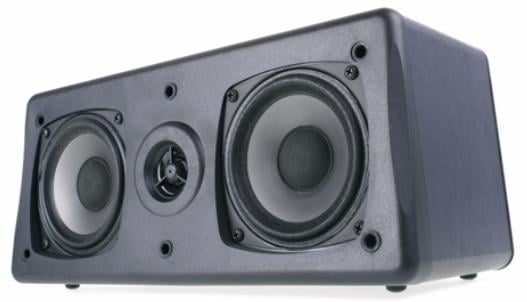
achieving the targeted maximum sound pressure level. The common approach is to then double up the
midrange drivers, splitting the workload into two. This results in a speaker that’s wide, not
very tall, and as we will see, often compromised with respect to redundant
driver wave interference. Throughout
this article we’ll refer to these designs as they are horizontally designed by
their driver types. The most common
design is a midrange-tweeter-midrange or MTM as we’ll call it.
With their height constrained, center channels still need to
reproduce all that mostly-vocal content with dynamics and clarity, down to 80
Hz or lower until the subwoofer takes over the heavy lifting. Most center channels try to be five to eight
inches tall, which results in their midrange drivers being restricted to four,
five, or six inches in diameter. To get
four to six inch drivers to dynamically reproduce 80 Hz starts getting very
expensive, if not practically impossible for minimizing distortion and
achieving the targeted maximum sound pressure level. The common approach is to then double up the
midrange drivers, splitting the workload into two. This results in a speaker that’s wide, not
very tall, and as we will see, often compromised with respect to redundant
driver wave interference. Throughout
this article we’ll refer to these designs as they are horizontally designed by
their driver types. The most common
design is a midrange-tweeter-midrange or MTM as we’ll call it.
 If anyone likes you enough
to watch a movie with you, the center channel must reproduce all that content
smoothly and predictably across all your seats.
If you’re sitting perfectly in front of the center channel, having
multiple drivers of the same type in a horizontal configuration can do the job
just fine. But if you move slightly
off-axis, or as any of the other seats will realize, having
horizontally-aligned redundant drivers will cause some frequencies to be
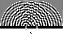
canceled and some to be reinforced. This
phenomenon is called wave
interference and you can read more about a double-slit experiment with
light (or any other physical media that behaves in waves) here. The subtracting and adding of various
frequencies at various angles can result in audible shifting in the speaker’s
sound across the room. Not only does the
off-axis frequency response suffer, but timing and phase response follow. Off-axis, MTM speakers can often sound hollow
but the comb filtering, or lobing effect, can also shift the imaging away from
the middle as a “phasy” sound. There’s a
good reason why one-piece surround speakers use a lot of identical drivers (up
to 40 - wow). The wave interference in
those cases is used as a tool of good, not evil. To compensate for the lack of intelligibility
(of the audio, not the script), people typically turn their volumes up which
then can then result in some domestic tension among spouses, children and
neighbors.
If anyone likes you enough
to watch a movie with you, the center channel must reproduce all that content
smoothly and predictably across all your seats.
If you’re sitting perfectly in front of the center channel, having
multiple drivers of the same type in a horizontal configuration can do the job
just fine. But if you move slightly
off-axis, or as any of the other seats will realize, having
horizontally-aligned redundant drivers will cause some frequencies to be
canceled and some to be reinforced. This
phenomenon is called wave
interference and you can read more about a double-slit experiment with
light (or any other physical media that behaves in waves) here. The subtracting and adding of various
frequencies at various angles can result in audible shifting in the speaker’s
sound across the room. Not only does the
off-axis frequency response suffer, but timing and phase response follow. Off-axis, MTM speakers can often sound hollow
but the comb filtering, or lobing effect, can also shift the imaging away from
the middle as a “phasy” sound. There’s a
good reason why one-piece surround speakers use a lot of identical drivers (up
to 40 - wow). The wave interference in
those cases is used as a tool of good, not evil. To compensate for the lack of intelligibility
(of the audio, not the script), people typically turn their volumes up which
then can then result in some domestic tension among spouses, children and
neighbors.
Floor speakers with multiple vertical redundant drivers will also have wave interference, but vertical variation in frequency response is much less of a problem than horizontal variation. In fact, the more identical drivers a loudspeaker has, the more it behaves like a line source instead of a point source. Line sources radiate in a more cylindrical pattern, which is advantageous if it is vertically oriented, as line sources interact less with the floor and ceiling. But a cylindrical radiation pattern is a disadvantage if you arrange the redundant drivers horizontally. The speaker will then interact more with the floor and ceiling, and suffer poorer response horizontally across the room.
We’re going to look at several design options, and zero in on what effects result from having multiple redundant drivers aligned horizontally. We’ll compare MTM designs with their bookshelf brethrens, see how designers can reduce the wave interference to a very minor effect, as well as explore some less common ideas to drive home the point and provide emotional drama. Improving your center channel performance can dramatically improve your overall sound, and as we’ll see can be done better with less money.
Test Setup and Methodology
To focus on the off-axis frequency variation in different speaker designs, I needed to take many measurements across different angles, map and analyze their results. In these tests I rotate the speaker instead of moving the microphone, as I don’t want to measure the acoustical differences across the room, another huge source of frequency variation as you move through the peaks and nulls of room modes and reflections. The walls have their first reflection points treated with 4 inch thick absorption and are at least eight feet away from the tripod where the speakers will rest. The Infinity IRS Epsilon I use as a center channel is about two feet behind the speaker. The red dot in some pictures is from the laser pointer to assure I have the calibrated Behringer ECM8000 microphone perfectly aimed, which is placed 11 feet from the speaker.
I played pink noise through each speaker and mapped its frequency response every five degrees from zero to 40 degrees off axis with 1/24 octave resolution. I’m assuming that the response is symmetrical, so I only measured one side for the analysis. The results below 80 Hz, a common and typically good crossover frequency to your subwoofer, and above 20 kHz were discarded. I’ll show the frequency maps of the speakers across their entire 80 to 20k bandwidth, but will focus on the frequency range of redundant drivers and measure their frequency variation as we vary the angle. All frequency responses were normalized for their zero-degree measurement. This article doesn’t care about and won’t show the absolute frequency response; you’ll select the sound quality of the speaker based on your budget and personal preferences. Instead, I just wanted to know what the change is from The Captain’s Chair to the other typically unlucky listeners. None of the speakers will have their grills attached, both to maintain some degree of anonymity but to also keep the photos and measurements as clear as possible.
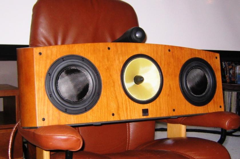
$250 MTM Horizontally Oriented Measurements
 The first speaker we’ll
look at is a very common MTM design, available from a big box retailer where
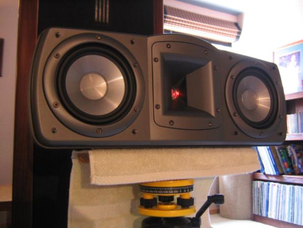
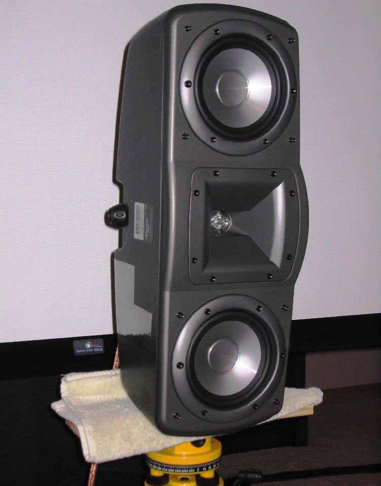
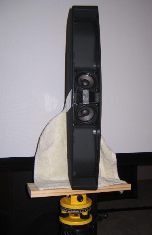
you can reportedly get some best buys. The
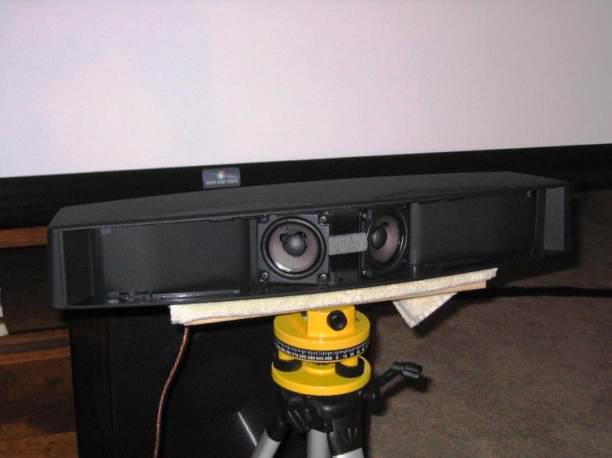
picture shows the speaker horizontally placed on a tripod with angle markings
so I can accurately measure the speaker’s off-axis response. The horn-loaded tweeter crosses over to the
dual 5.25 inch midrange drivers at 2400 Hz.
This means that while we will see the performance of the tweeter’s
off-axis response, we will focus our analysis in the bandwidth of 80 to 2400
Hz.
The first speaker we’ll
look at is a very common MTM design, available from a big box retailer where
you can reportedly get some best buys. The
picture shows the speaker horizontally placed on a tripod with angle markings
so I can accurately measure the speaker’s off-axis response. The horn-loaded tweeter crosses over to the
dual 5.25 inch midrange drivers at 2400 Hz.
This means that while we will see the performance of the tweeter’s
off-axis response, we will focus our analysis in the bandwidth of 80 to 2400
Hz.
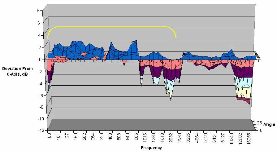
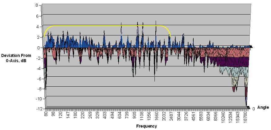
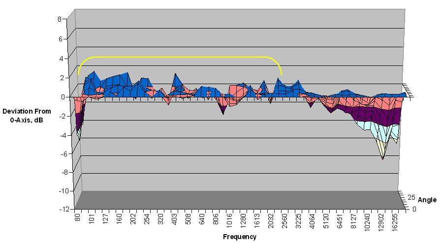
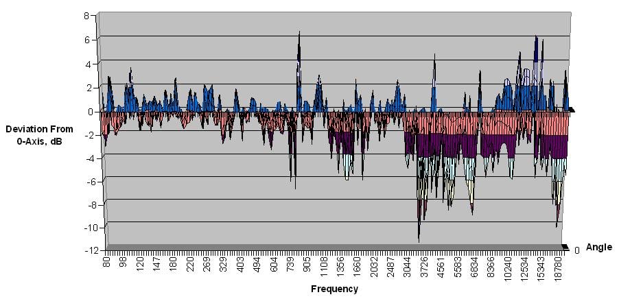
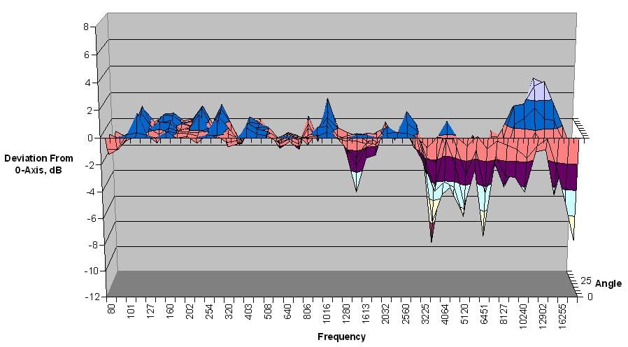
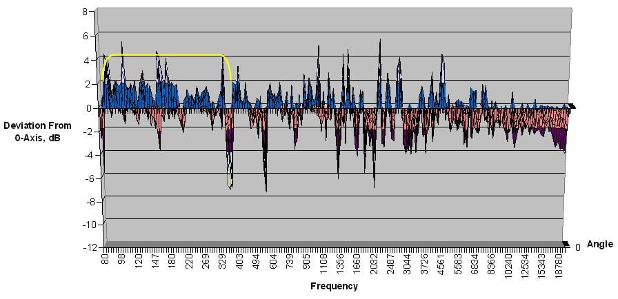
In the chart below, the frequency response of this MTM center channel was mapped with 1/24 resolution, from 80 to 20,000 Hz in the x axis and from zero to 40 degrees angle in the z axis (front to back). The initial response on axis was normalized so the measurement you see in the chart is the deviation from the on-axis response as the angle of the speaker was changed. You can see a significant change in frequency response in the top octave, but we’re not here to pick on the off-axis response of this speaker’s horn tweeter, as terrible as it is. What we are here to pick on is the frequencies that the two “Ms” are reproducing, from 80 to 2400 Hz, which is shown with the yellow bracket. In this zone the measurements show peaks of over four dB from the additive effect of the two midranges and wave cancellation of over -10 dB.
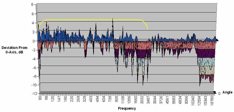
The 1/24 octave chart above looks pretty messy. However, the peaks and troughs are less audible the narrower they are because your hearing will naturally smooth out the response. Plus or minus a couple dB also isn’t anything to lose sleep about, but what we can see from the chart is that the two midrange drivers exhibit significant wave cancellation from around 800 Hz to where the crossover kicks in at 2400 Hz. Some of the variation near the crossover point is from all three drivers playing the same frequencies. A higher-order crossover would reduce this problem, but just placing the tweeter above the midrange would fix it completely as we’ll see later on.
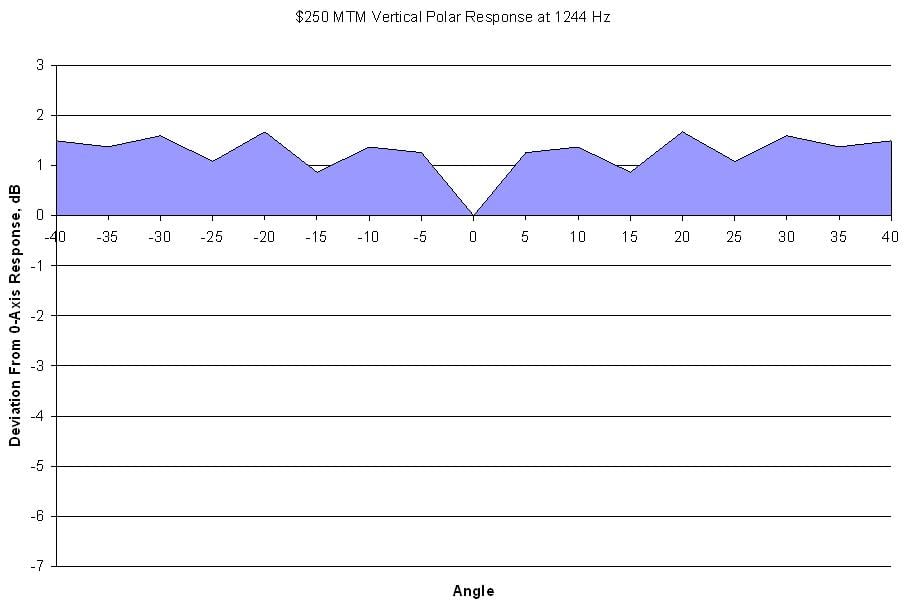
If we take a slice of one frequency from the 1/24 octave measurements we can plot out the frequency response of the loudspeaker and get a visual representation of lobing. The lobing effect is from the appearance on a polar map of the peaks and valleys of the frequency response. In a real polar graph, it looks like lobes, or flower petals. This chart is a bit simpler, as I only measured an 80 degree angle (assumed to be symmetrical) and am using a more traditional chart.
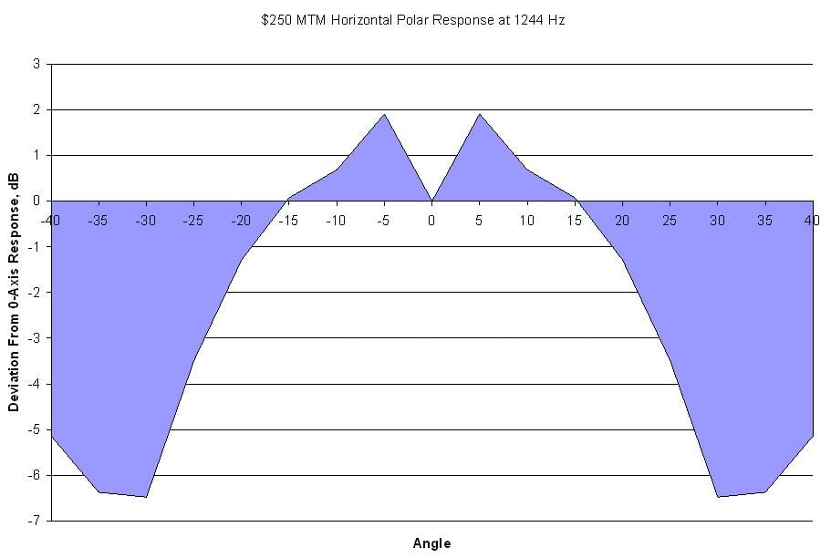
Conventional wisdom is that people typically can’t differentiate frequency changes finer than 1/3 octave, but I argue that is a bit too course a guideline to follow. In my experience, 1/6 octave smoothing is a more appropriate method to determine audibility of frequency responses. In order to better chart the audible effects of the wave interference, the chart below shows the same measurements but averaged at a 1/6 octave resolution. This chart indicates the significant, and audible, wave cancellation in the upper midrange. When the variation from on-axis response, from 80 to 2400 Hz is calculated using standard deviation, this speaker gets a score of 1.94. We’ll see later how that compares to other types of center channels.
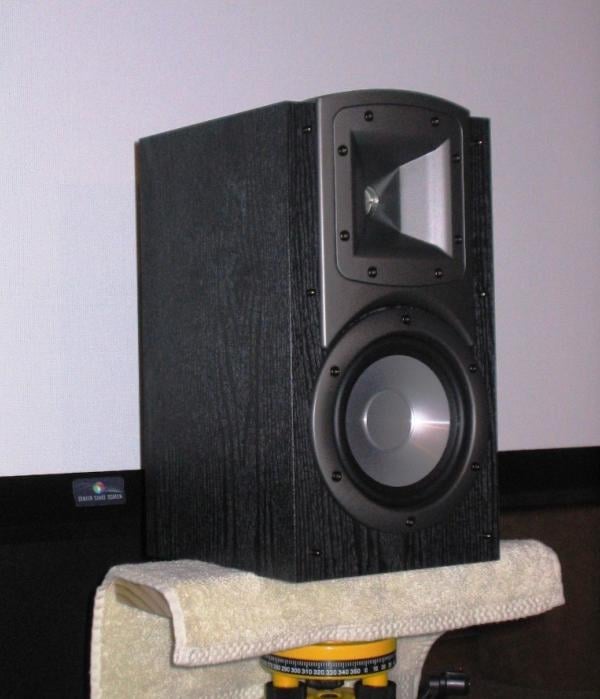
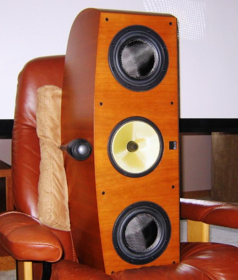
$250 MTM Vertically Oriented Measurements
 What would happen if we
take that MTM speaker and turned it on its side? I did just that, by modifying my high-tech
stand with another piece of wood and some tape.
It may not be pretty but it’s for the science, right? I dropped a Center Stage acoustically transparent
screen down behind the speaker. It
didn’t affect the acoustics and I could get better photos.
What would happen if we
take that MTM speaker and turned it on its side? I did just that, by modifying my high-tech
stand with another piece of wood and some tape.
It may not be pretty but it’s for the science, right? I dropped a Center Stage acoustically transparent
screen down behind the speaker. It
didn’t affect the acoustics and I could get better photos.
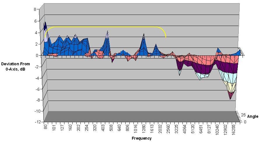
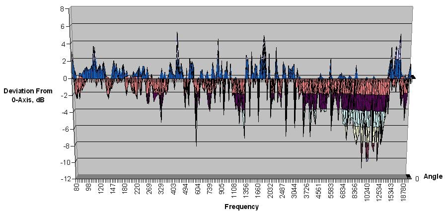
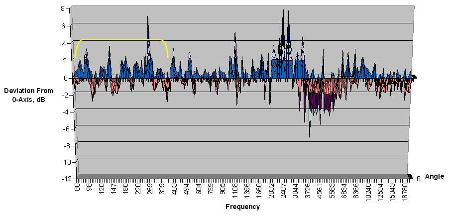
In the 1/24 octave chart below, we can see the effect from rotating this speaker vertically. The horn tweeter isn’t as happy, exhibiting worse off-axis response from 4 k to 10 kHz, but you can see the frequency response from the midrange drivers shows much less wave interference.
If we look at the same slice at 1244 Hz to compare its lobing to the horizontal orientation, you can see from the below chart that for the specific frequency it was successfully eliminated. I won’t be showing any more of these charts because while they show the lobing shape more clearly, the 3D charts have more color. That must be a good thing.
To better gauge the audibility of orientating the speaker vertically, the chart below shows the measurements with 1/6 octave smoothing. The horn is clearly not designed to be rotated 90 degrees, but by not having horizontally arraigned redundant drivers, we have improved the smoothness of the speaker’s off-axis response a great deal. In the midrange drivers’ frequencies, the standard deviation improved to 1.19.
$115 Bookshelf Speaker Measurements
 This company’s horn tweeter
should be used in the orientation as it was designed, but if you were keen on
using their speakers, how would you avoid the wave interference that the
horizontally aligned MTM center channel had?
One solution is to completely avoid their center channel and use a
bookshelf speaker, hopefully one that’s identical to your left and right
speakers. With this configuration, you
get a properly oriented horn as well as a much smoother frequency response
across the room. The price is $230 for a
pair, so depending on if you can find any use for the other bookshelf or not,
you just saved yourself from $20 to $135 and got better sound to boot. Cheaper and better? Win, win, and win.
This company’s horn tweeter
should be used in the orientation as it was designed, but if you were keen on
using their speakers, how would you avoid the wave interference that the
horizontally aligned MTM center channel had?
One solution is to completely avoid their center channel and use a
bookshelf speaker, hopefully one that’s identical to your left and right
speakers. With this configuration, you
get a properly oriented horn as well as a much smoother frequency response
across the room. The price is $230 for a
pair, so depending on if you can find any use for the other bookshelf or not,
you just saved yourself from $20 to $135 and got better sound to boot. Cheaper and better? Win, win, and win.
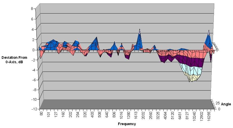
Below is the chart showing the frequency response deviation from on-axis to 40 degrees off-axis. The chart shows the same off-axis roughness of the tweeter, but there may be other reasons why you would otherwise like the speaker’s sound. Importantly to this endeavor, the midrange doesn’t show any significant change in frequency response at different angles.
The 1/6 octave chart below shows that the bookshelf speaker performs very well off-axis by only having one midrange driver. For comparison’s sake, we will focus on the same frequency range of the midrange and score the variation. The average standard deviation of the frequency with respect to angle for the bookshelf is 1.01.
So what have we figured out thus far? First, that the horizontally oriented MTM center channel has significant variation in frequency response at different angles. Second, that by vertically orienting the MTM speaker we were able to significantly reduce the variation, but this company’s horn performance suffers and otherwise compromises this plan. And third, the smoothest response and less expensive bookshelf performs better, while possibly matching your left and right channels with complete perfection.
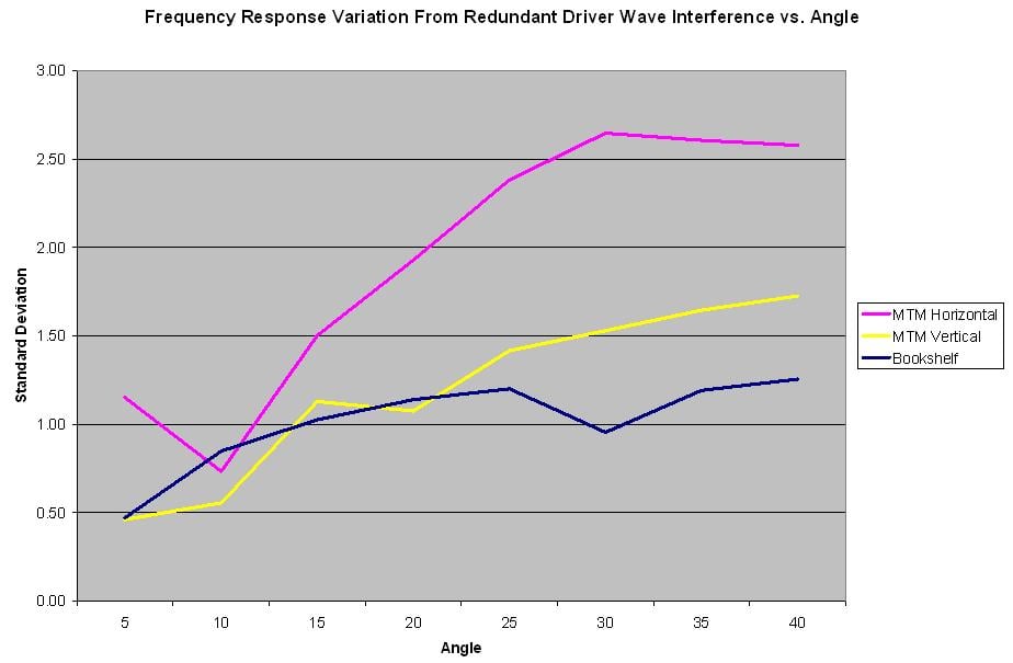
If we compare their standard deviations at different angles, we can get an idea of the variation or roughness in the 1/6 octave frequency response. In the chart below, the three configurations are graphed with their standard deviations. Lower scores are better. Clearly, if one were shopping for a surround sound system from this company, the better performing, better value choice would be to use three identical bookshelf speakers across the front soundstage.
|
|
Average Frequency
Variation From 0-Axis, |
|
$250 MTM Horizontal Center |
1.94 |
|
$250 MTM Vertical Center |
1.19 |
|
$115 ($230) Bookshelf |
1.01 |
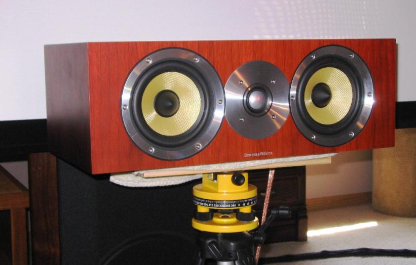
$199 MMMM Horizontally Oriented Measurements
 If you were setting out to
design a speaker with the worst off-axis response possible, you should use a
whole bunch of identical horizontal drivers.
This next center channel speaker does mostly that, with four identical
“full range” 2.5 inch paper drivers, two in the front and two inside to help
load their ported enclosure. It could be
said that this speaker “has no highs, has no lows, must be…”, but because the
front two drivers are oriented at an angle from each other, this speaker
maintains its mediocrity with a fair degree of consistency. This company’s ad copy states that their
design “’locks’ dramatic dialogue to the screen.” If by this they mean that their design
diffuses dialogue across your room, they would be right on.
If you were setting out to
design a speaker with the worst off-axis response possible, you should use a
whole bunch of identical horizontal drivers.
This next center channel speaker does mostly that, with four identical
“full range” 2.5 inch paper drivers, two in the front and two inside to help
load their ported enclosure. It could be
said that this speaker “has no highs, has no lows, must be…”, but because the
front two drivers are oriented at an angle from each other, this speaker
maintains its mediocrity with a fair degree of consistency. This company’s ad copy states that their
design “’locks’ dramatic dialogue to the screen.” If by this they mean that their design
diffuses dialogue across your room, they would be right on.
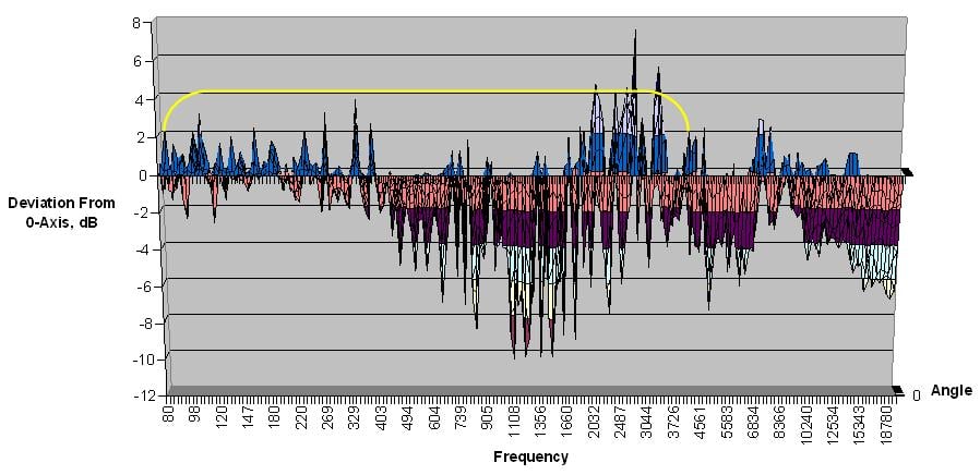
In the 1/24 octave chart below, you can see severe wave interference in the top three octaves (2.5 to 20 kHz), as well as some trouble in the upper midrange (1.3 to 1.8 kHz). Most of the narrowest spikes are inaudible in practice, so we’ll need to smooth out this data a bit and calculate how much the frequency response varies from the normalized on-axis measurement.
In the 1/6 octave chart below we can see that the wave interference is quite audible around 1.4 kHz and becomes severe above 2.5 kHz. This charts shows that there are angles at which you can get over 10 dB of wave cancellation in the frequencies that are critical for vocal intelligibility. A 10 dB loss of significant portions of the lower treble would be perceived as being half as loud. The biggest problem is that the behavior is not linear or predictable. You can’t just turn the volume up to compensate for the low fidelity sound that the other seats would experience.
Around 20 degrees off-axis of the loudspeaker, one becomes on-axis to one of the angled “full-range” drivers. When you get on-axis with one of these beauties, the high frequency beaming that occurs from trying to make a 2.5 inch driver into a tweeter becomes apparent. There is an audible peak around 11 kHz when you’re directly in front of a driver, which would sound sibilant and tizzy. Combine that harshness with the loss of lower treble and upper midrange that brings presence and intelligibility, and you’ll be undermining the entire experience. Disappointing the spouse won’t help your next request for spending the family budget on “what is it you want now?”
The best way to minimize wave interference is to minimize the frequency range that redundant horizontal drivers reproduce. This MMMM speaker (or is it a FF?) doesn’t relieve the drivers with a crossover, and so we have to calculate and score its variation in horizontal frequency response from 80 Hz to 20 kHz, which comes out at 1.81.
$199 MMMM Vertically Oriented Measurements
 The question remains as to how much of the variation in
horizontal frequency response is due to wave interference between the drivers,
versus the natural off-axis response of the driver itself. To answer this, we then turned the speaker on
its side and measured how well it performed off-axis with the wave interference
essentially taken out of the equation.
The question remains as to how much of the variation in
horizontal frequency response is due to wave interference between the drivers,
versus the natural off-axis response of the driver itself. To answer this, we then turned the speaker on
its side and measured how well it performed off-axis with the wave interference
essentially taken out of the equation.
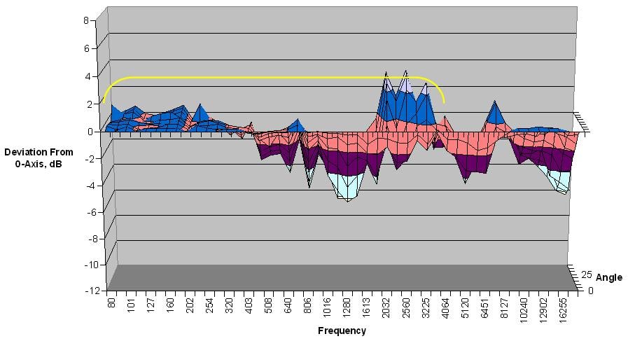
In the 1/24 octave chart below, it looks perhaps a bit better but very similar to what we originally measured. We’ll have to look at the 1/6 octave chart and standard deviation to see how much good this does.
In the 1/6 octave chart below, you can see that we essentially eliminated the upper midrange null around 1.5 kHz. The null was around -6 dB, which is quite audible, and when oriented vertically you can see all the variation is less than +/-2 dB with the exception of one frequency that increases to +4 dB. The lower treble performance is arguably better. The off-axis attenuation occurs at slightly higher frequencies, but is still an ugly mess, swallowing -8 dB of dialogue-critical treble. The 11 kHz tizzy spike is tamed down somewhat. Overall, the vertical orientation slightly improved the frequency variation, but not by much. The standard deviation of its radiation pattern improved only to 1.64. The majority of this speaker’s problems are with the radiation patterns and orientation of the drivers themselves. Starting with drivers like these, the speaker designer is for the most part doomed from the beginning.
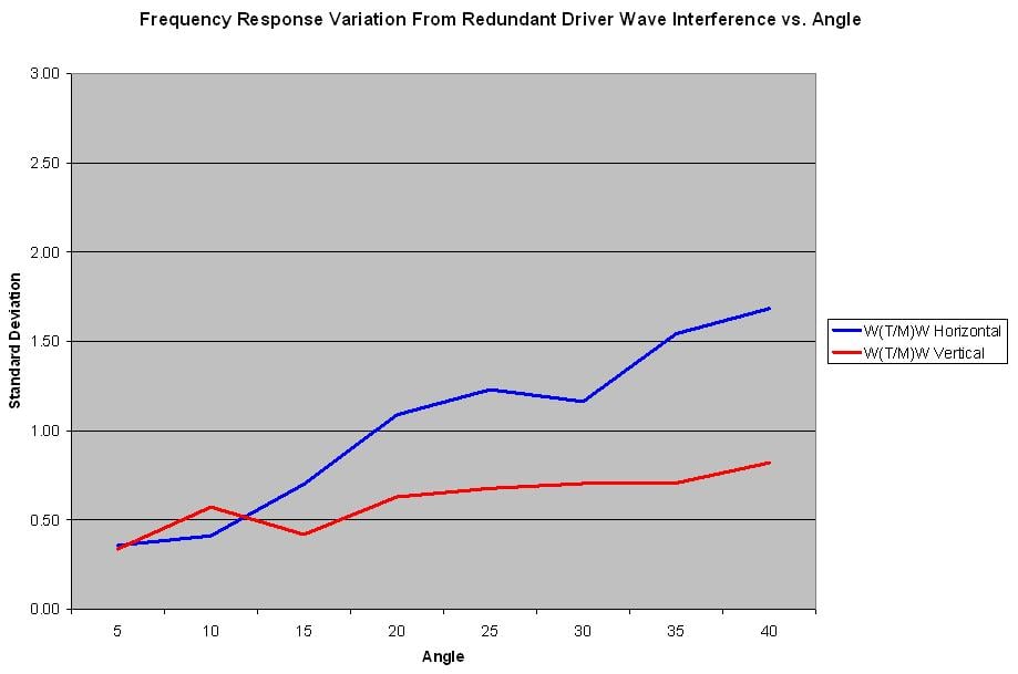
In the chart below, you can see a comparison of how much variation the speaker had horizontally and vertically, and how they were related to angle. You can see that up to 20 degrees off-axis, the speaker performed better by having its drivers oriented vertically. Again, a lower standard deviation means less variation in frequency response. However, at angles greater than 25 degrees the angled front baffle was clearly worse off being turned vertically. There are several floor-standing loudspeaker designs that focus a vertical array towards the listener in the center plane, and you can see from these measurements why you wouldn’t do the opposite.
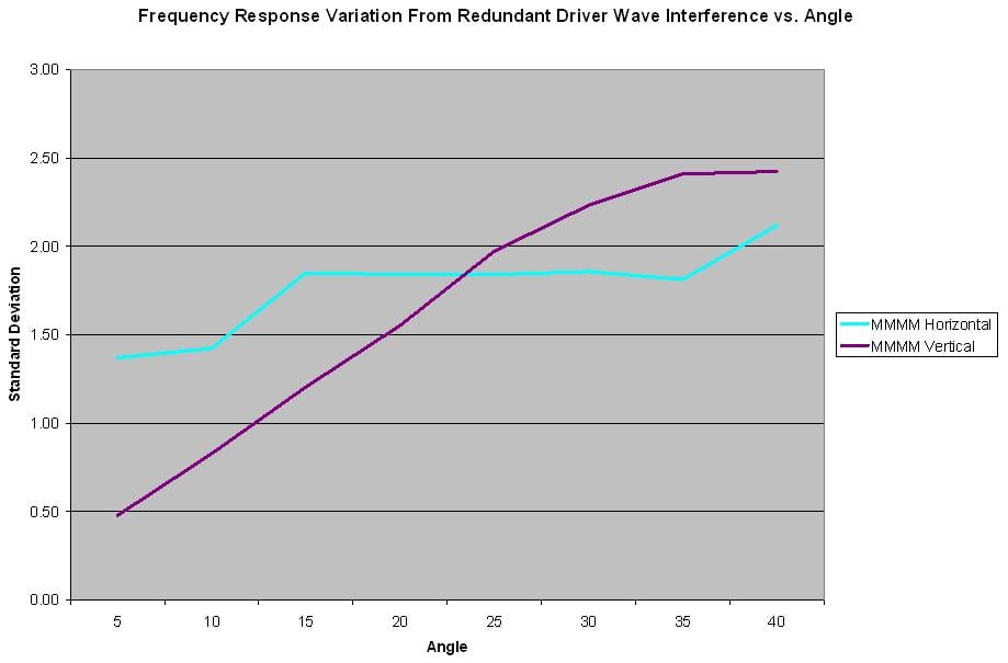
If you were shopping for a surround sound system from this company, you would be doing slightly better by orienting the speaker vertically and would presumably do better using a center channel that’s identical to your left/ right channels. But the driver performances are so bad, that it mostly doesn’t matter what you do. You could turn the speaker completely around or put it in the closet and it won’t get much worse.
|
|
Average
Frequency Variation From 0-Axis, |
|
$199 MMMM Horizontal Center |
1.77 |
|
$199 MMMM Vertical Center |
1.64 |
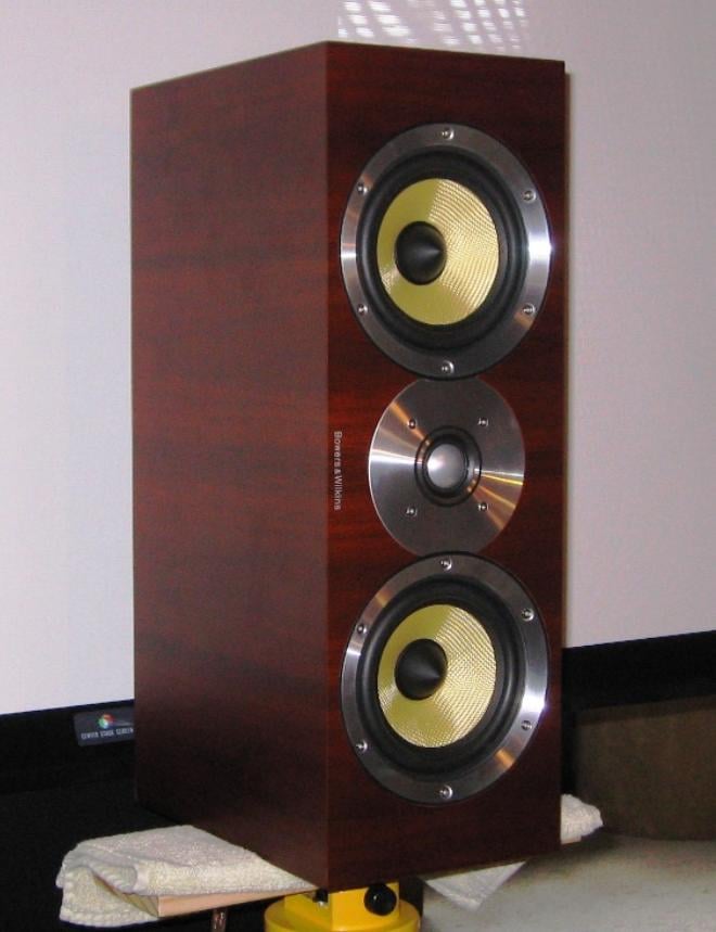
$600 MTM Horizontally Oriented Measurements
 This is one beautiful speaker. Naturally, we wanted to look at higher-end
designs and see to what degree higher quality drivers improve the overall
response versus what if any limitations these more expensive speakers have with
wave interference. This traditional MTM
design has the crossover point at 4 kHz, which is rather high. This unfortunately increases the frequency
areas where the two midrange drivers are interfering with each other, but at
this point we can just assume. Let’s turn
to the charts to see what we get for our hard earned 600 dollars.
This is one beautiful speaker. Naturally, we wanted to look at higher-end
designs and see to what degree higher quality drivers improve the overall
response versus what if any limitations these more expensive speakers have with
wave interference. This traditional MTM
design has the crossover point at 4 kHz, which is rather high. This unfortunately increases the frequency
areas where the two midrange drivers are interfering with each other, but at
this point we can just assume. Let’s turn
to the charts to see what we get for our hard earned 600 dollars.
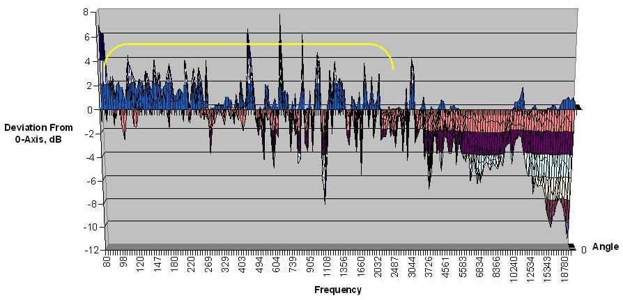
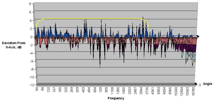
In the 1/24 octave chart below you can see some significant wave interference, ranging from +8 dB additive to -10 dB of cancellation. The frequency range where the two midrange drivers would be interfering with each other is highlighted by the yellow bracket. The variation in this range is where we will also be scoring the speaker and comparing against other configurations.
In the 1/6 octave chart below, you can see that the interference between the two midrange drivers is audible. In the upper midrange we can see over -6 dB of cancellation and almost 4 dB of wave reinforcement. You can also see the tweeter has audible off-axis attenuation, but it’s important to emphasize that these tests only reflect variation from the on-axis response and how well we can avoid wave interference. This speaker series has a wonderfully musical sound quality, and I’d take rolled-off beautiful over well-dispersed junk any day.
When the variation of the frequency is calculated at various angles, the average standard deviation of this MTM speaker, from 80 Hz to 4 kHz is 1.62. It’s a beautiful and musical speaker, but the off-axis response of the midrange drivers is mediocre. In this design, the midrange drivers reproduce over five octaves compared to the tweeter’s two, so let’s see if we can improve things by rotating it.
$600 MTM Vertically Oriented Measurements
 In order to easily test if
the drivers or cabinet are primarily to blame for the off-axis response, or if
the MTM configuration itself is the limiting aspect, we then rotated the
speaker vertically and ran it through another set of measurements. Fortunately, this speaker’s cabinet is square
on the ends and this is actually a possible mounting configuration for your
home theater. Would it improve the
frequency response?
In order to easily test if
the drivers or cabinet are primarily to blame for the off-axis response, or if
the MTM configuration itself is the limiting aspect, we then rotated the
speaker vertically and ran it through another set of measurements. Fortunately, this speaker’s cabinet is square
on the ends and this is actually a possible mounting configuration for your
home theater. Would it improve the
frequency response?
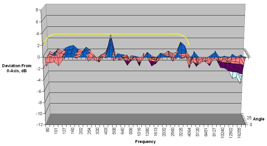
In the 1/24 octave chart below, it is easy to see that we significantly improved the off-axis midrange response by vertically orienting the speaker. Any peaks in the midrange are very narrow, which is just the way they should be. There is still some off-axis attenuation to the tweeter, but it has also been improved.
In the 1/6 octave chart below, you can see that the wave interference from the two midrange drivers was virtually eliminated. The off-axis response is smooth and consistent up to 40 degrees off axis. The lower treble from the tweeter has even improved, likely due to it now having a narrow horizontal baffle and reduced cabinet diffraction. In this orientation, this speaker would do a terrific job at maintaining intelligibility and clarity across your room. This is the type of performance that truthfully “locks dramatic dialogue to the screen.”
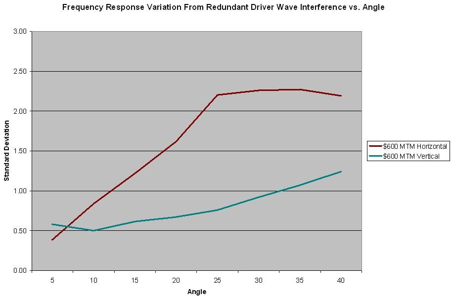
If the variation in frequency response is calculated in the vertical orientation, this speaker scores an average 0.80. Vertically orienting this speaker cut the variation in frequency response by nearly one standard deviation. The chart below shows the center speaker’s off-axis variation in relation to angle. The vertical orientation showed a significantly reduced variation in frequency response.
|
|
Average Frequency Variation From 0-Axis, 80-4000 Hz, (Lower is Better) |
|
$600 MTM Horizontal Center |
1.62 |
|
$600 MTM Vertical Center |
0.80 |
With a nice set of speaker stands or brackets, three of these beauties vertically oriented would create a great front soundstage. Or, another option would be three of their bookshelf speakers across the front. This company’s matching bookshelf speaker lists for $900 for a pair, so in theory you could once again save money and get better sound for your guests by avoiding the center speaker design. Unfortunately, this company – like most – doesn’t offer their stereo speakers individually, so unless you can find another use for the other speaker, buying three identical speakers for the front isn’t easy. For this product line, three vertically-oriented center channels would be your least-expensive, highest-performance standard option.
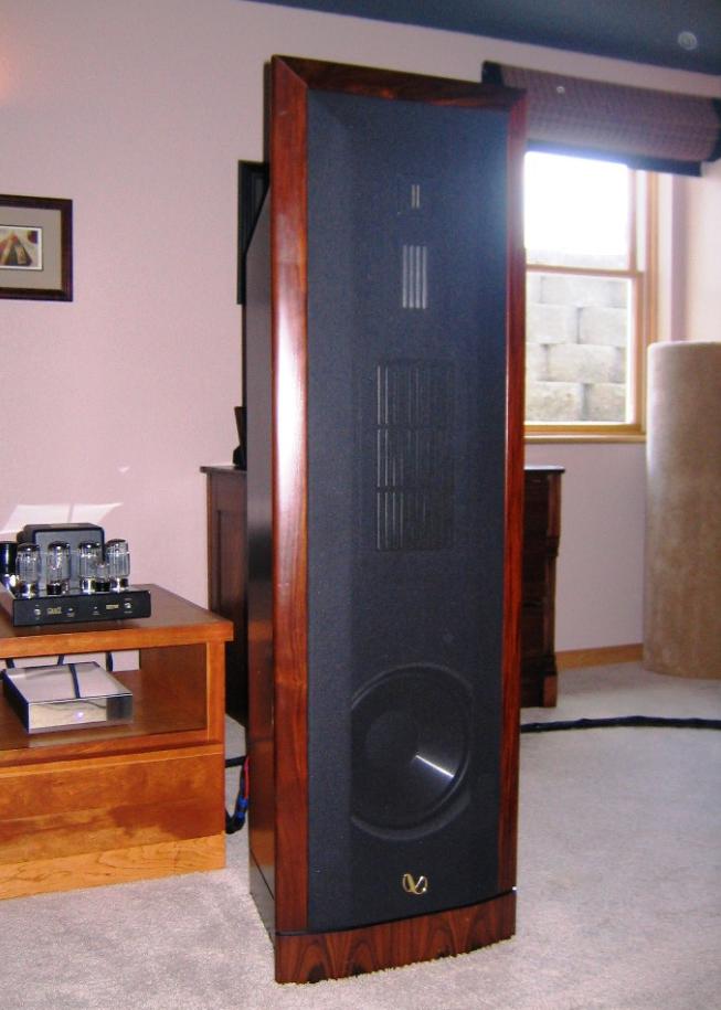
$2500 WTMW Horizontally Oriented
 Now we get to take a peak
at a very high-end center speaker design.
Since this large speaker easily outgrew my test stand, it gets to rest
in The Captain’s Chair for this test, receiving better treatment than most of
my family. The Stressless® Recliner
naturally cradled the speaker in all of its supple softness, which certainly
resulted in a less stressed sound.
Now we get to take a peak
at a very high-end center speaker design.
Since this large speaker easily outgrew my test stand, it gets to rest
in The Captain’s Chair for this test, receiving better treatment than most of
my family. The Stressless® Recliner
naturally cradled the speaker in all of its supple softness, which certainly
resulted in a less stressed sound.
This $2500 supermodel maintains a mostly horizontal profile, while reducing potential wave interference by having less of the bandwidth play through horizontally redundant drivers. Speakers that have the tweeter and midrange vertically arranged will naturally have a smoother off-axis response. To supplement the dynamic headroom of this speaker and allow you to lower your subwoofer crossover point (although there are good arguments to keep it at 80 Hz), this design has two woofers that are low-pass filtered at 350 Hz.
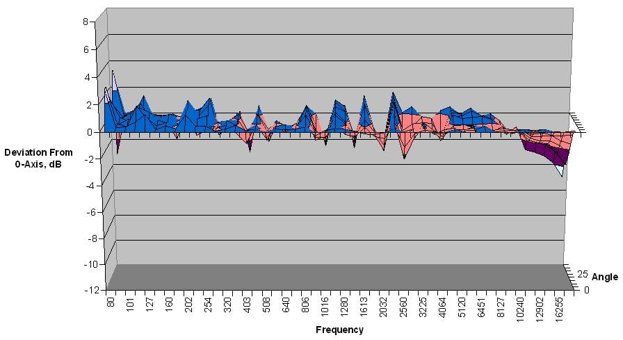
The 1/24 octave chart below shows a generally inaudible difference in the speaker’s response across various angles. The frequency range of the redundant drivers, from 80 to 350 Hz, is highlighted by the yellow bracket.
In the 1/6 octave chart below, the off-axis response of this speaker was nearly perfect. We can see one significant -5 dB wave cancellation from the woofers interfering with each other just above their crossover point at 360 Hz. Even though this would be audible, because the entire effect is such a narrow bandwidth, this really isn’t something to worry about. The off-axis response of the tweeter is fantastic.

The standard deviation of the frequency response from the two woofers calculated to 1.02. This was by far the best performing horizontally oriented configuration.
$2500 WTMW Vertically Oriented
 To experiment with this heavyweight
in a vertical orientation, it not only required The Captain’s Chair, but also
The Comfy Pillow. Naturally, I assume
the pillow further reduced any stresses the speaker would feel. I was going to draw the line if it also
needed slippers and a paper, but it turned out the only additional effort I
needed was to endure the well-deserved ribbing from onlookers. This design doesn’t have square ends, so
you’d never want to do this permanently, but let’s see what happens.
To experiment with this heavyweight
in a vertical orientation, it not only required The Captain’s Chair, but also
The Comfy Pillow. Naturally, I assume
the pillow further reduced any stresses the speaker would feel. I was going to draw the line if it also
needed slippers and a paper, but it turned out the only additional effort I
needed was to endure the well-deserved ribbing from onlookers. This design doesn’t have square ends, so
you’d never want to do this permanently, but let’s see what happens.
In the 1/24 octave chart below, you can see that something is worse in the upper midrange and lower treble. With the tweeter and midrange arranged horizontally you can now see the wave interference above and below the 4 kHz crossover point. This company uses a first-order crossover between their tweeter and midrange, which means that there are about two octaves where there the two drivers interact with each other. If vertically aligned, this wouldn’t be an issue and their integration of the two drivers sounds absolutely perfect. None of their speakers are meant to have a horizontal tweeter-midrange arrangement like this, and their top models don’t even place the midrange in the same baffle as the woofers.
In the 1/6 octave chart below, you can more clearly see the audible performance of this well-pampered configuration. By vertically orienting it, we have successfully eliminated the wave interference of the two woofers just above their crossover point at 360 Hz. However, like we saw in the horn-tweeter design, this speaker is clearly not designed to be positioned like this. The first-order tweeter crossover is audibly allowing wave interference to occur for an octave above and below the crossover point. We’ve fixed a minor wave interference problem but created another which is much worse. If only they had a center speaker that had all the drivers arranged vertically… oh wait, they call those “main” speakers. Unfortunately, many people are stuck in the mindset that the center channel must only use a special center speaker design. In reality, there are often better options, but because this speaker only has a couple octaves where the drivers are redundant, this design isn’t that compromised.
The wave interference from the woofers was clearly improved by vertically orienting the speaker. The standard deviation in the woofers’ range of 80 to 350 Hz was calculated to be 0.61. The inter-driver interference we created between the tweeter and midrange isn’t included in this score. Including crossover effects and inherent driver radiation patterns (e.g. the horn tweeter in Part 1) would increase the scope too much. I wanted to focus as tightly as reasonable on just the interaction between horizontally arranged redundant drivers.
|
|
Average
Frequency Variation From 0-Axis, |
|
$2600 W(T/M)W Horizontal Center |
1.02 |
|
$2600 W(T/M)W Vertical Center |
0.61 |
While the woofer wave interference was practically eliminated by rotating this speaker vertically, there are many reasons why you wouldn’t want to do this for this design. However, having shown that one type of sonic compromise can be avoided by thinking vertically it would be wise to pursue using three identical “main” speakers across your front soundstage. Their floor standing speaker with identical drivers and crossover points retail at $4000 for the pair, so again in theory you could get better sound at a lower cost if this company sold them individually. I know that one high-end multichannel audio reviewer I follow uses three of this company’s floor standing speakers across his front soundstage.
In the manufacturer’s main brochure on this series, they proudly show off how Skywalker Sound uses three identical floor-standing “main” speakers across their front soundstage. It’s curious that while configurations like this are correctly portrayed as achieving the highest multichannel front soundstage possible, the company only sells their main speakers in pairs. Maybe Lucas just threw the extra in the closet.
On one hand, this center channel design avoids wave interference very reasonably. However on the other hand people in this price point are keenly interested in getting the best sound possible.
Conclusion, Rankings and Evaluation
In every case where we measured a center channel speaker with redundant horizontal drivers we were able to improve the smoothness of its horizontal frequency response in that range by reorienting the speaker vertically. While only the $600 MTM was symmetrical enough to be universally improved by using it vertically, we can clearly see the wave interference in the designs and ways to avoid it.
|
Center Speaker Ranking |
Average
Frequency Variation From 0-Axis Due to Wave Interference, Standard Deviation, |
|
$2500 W(T/M)W Vertical |
0.61 |
|
$600 MTM Vertical |
0.80 |
|
$115 Bookshelf |
1.01 |
|
$2500 W(T/M)W Horizontal |
1.02 |
|
$250 MTM Vertical |
1.19 |
|
$600 MTM Horizontal |
1.62 |
|
$199 MMMM Vertical |
1.6 |
|
$199 MMMM Horizontal |
1.77 |
|
$250 MTM Horizontal |
1.94 |
To get the most cohesive performance out of perhaps the most important channel in your home theater, strive for getting a center channel that is identical to your mains. If you can’t accommodate that goal, then do your best to avoid or minimize wave interference across your room by being wary of horizontal redundancy. Look for designs that have a vertical arrangement of their tweeters and midrange drivers. Look for planar, coaxial, lower tweeter crossover points, higher order crossovers, or other designs that avoid or minimize the “double slit” effect and incoherency that can result. Perhaps you’ll find yourself buying a speaker with fewer, higher quality drivers. Perhaps you’ll save yourself some money. Perhaps you’ll find your guests enjoying what you’ve put together and happily encouraging you to spend more money on this family fun. That’s what we’re all really after, right?
Chris Seymour is owner of Seymour AV, an internet-direct manufacturer of “audiophile-first” audio and video equipment. Their first product is the Center Stage screen, an acoustically transparent, electrically retractable projection screen that offers a pure white image with positive gain at a reasonable price. Finally, audiophiles can get a screen that allows them to keep their sound.
Special thanks to who is perhaps the most impressive home theater dealer in the Midwest, Audio Video Logic. Ahead of their time, they’ve been demonstrating for years how you can often improve the sound of a center channel by simply rotating it vertically. They know first-hand the difficulties of countering myths such as “I can’t use that – it’s not a ‘center channel,’” and how to sympathetically counsel audiophiles into the intimidating world of home theater.
Addendum $7000 Tower Speaker
 I wasn’t interested in including my Infinity IRS Epsilon
that I use as a center channel in the results, because it:
I wasn’t interested in including my Infinity IRS Epsilon
that I use as a center channel in the results, because it:
- Doesn’t have any driver redundancy
- Isn’t horizontal without killing someone
- Lacks any similar model to compare it to, and
- Is not a design that is in current production (originally $14,000 per pair)
But while I had the test equipment setup, I was curious about how well it measured. Were my guests actually enjoying a coherent center channel sound, or were they just saying what they needed to get me to go away?
As you can see in the below 1/6 octave horizontal frequency response chart, the vertical array of drivers do not exhibit wave interference. There is a fall off in the top frequencies of the tweeter, which is common.
Infinity’s Cary Christie explained in his white paper on this speaker, “As the wavelengths approach the dimensions of the diaphragm, the waveshape begins to become planar rather than spherical. In a typical [one inch] dome tweeter, for example, this narrowing, or “beaming” becomes serious at about 10 kHz. If the dome had flat power response, the on-axis response would actually rise, and some do, however most show a roll-off in power response due to the reactive mass of the dome. The on-axis frequency response of such a tweeter may show a ‘flat’ characteristic out to beyond 20 kHz, but this is only because the energy is concentrated in an increasingly narrower angle. The actual power response of the dome is falling off rapidly, beginning its drop-off as low as 6 kHz.” The somewhat improved the off-axis response of this planar tweeter by adding a second one in the back. Even though this could in theory cause wave interference across the horizontal plane, the back tweeter’s response is randomized by reflecting off the back wall. My speakers are 6.7 feet from the back wall, which reduces the rear tweeter’s ability to help out. Regardless, I still have much more top frequency roll-off away from center than the W(T/M)W speaker that was used in configurations 8 and 9. My credit card just moaned.
From the test results, wave interference from redundant horizontal drivers or crossover overlap is not an issue. However well the Epsilon can possibly sound in The Captain’s Chair, it responds consistently across all seats in the room. My guests are surely experiencing as good a sound as my budget allowed for, but I’d guess they’re still appeasing me somewhat with acclaim. The last thing they’ll do is encourage me to spend more money.
They just don’t understand.