Lowering Mechanical Noise Floor in Speakers

When I design a loudspeaker system for home or studio use, with the goal of maximizing sonic accuracy, there are a handful of key areas I focus on when it comes time to judge how successful the design is.

Among the top three subjective criteria that I use in judging success in reaching the goal of sonic accuracy are soundstaging and transparency. Focusing on the latter, one of the things that I as the designer can do to maximize transparency is to lower the noise floor of the system - and do so as much as it is possible, given a particular design and budget constraints.

The test subject I'll be modeling is a system comprising a totally enclosed box. Its a mid-bass system, operating with a band pass response. The low pass -3dB point established by a crossover network at 430 Hz, with the particular driver/cabinet alignment chosen providing for a high pass -3dB point at 40 Hz.

The cabinet's panels will, virtually, be built of a polymer composite. I chose the composite, not only for its well-understood mechanical properties but also because of its strength, excellent dimensional stability and superior vibration damping properties.

Composite Sample Impulse Response

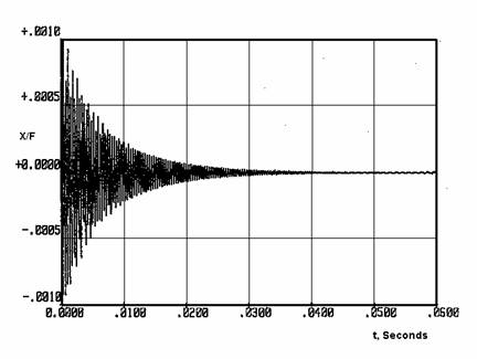
Indeed, the material I used for this model has the ability to dampen vibration 4 times faster than granite! Knuckle-rap a cabinet made of this composite and it feels - and sounds - as if you're knocking on a block of solid rock.

Panel acoustic output results from both varying internal surface pressure arising as a result of the action of the driver's diaphragm as well as mechanical vibration reaction induced by the motion of the driver's frame, as well as other panels. (The latter case is easy to envision when one considers the high degree of impedance matching that will exist between panels made of the same material unless measures are taken to provide for an impedance mismatch between the panels; doing so will reflect vibrational energy back to the source panel).

In either case, minimization of panel vibration can be accomplished by a variety of means including isolation, absorption, a combination of both or other such engineered solutions. In this first part of a 2-article series, I'll focus directly on the panels themselves and what can be done to minimize this sort of secondary acoustic radiation.

With these general design points in mind, let's commence the analysis.

Any panel, whether simply supported or clamped at any (or every) edge, will exhibit a clearly defined, vibrational mode series known as eigenvalue, which are theoretically infinite in number and, in general, are not harmonically related. To demonstrate this vibrational series, I ran a FEA (Finite Element Analysis) simulation, modeling a rectangular panel, clamped at all 4 edges, with the following physical dimensions:

Dimension	Named Variable	Value
Length	a	20" (.508 m)
Width	b	10" (.254 m)
Thickness	h	.75" (.01905 m)

The mechanical properties of the material, an isotropic polymer composite, are:

Properties	Metric Units	English Units
Density	2.32 g/cm^2	0.084 lb./in^3
Compressive Strength	110 - 117 MPa	16,000 - 17,000 psi
Tensile Strength	15.2 MPa	2,200 psi
Flexural Strength	17.2 MPa	2,500 psi
Young's Modulus	35,982 MPa	5.23E6 psi
Poisson's Ratio	0.23	0.23
Thermal Expansion	16.9E-6 mm/mm/ ˚ C	9.4E-6 in/in/ ˚ F
Thermal Conductivity	0.244 W cm/ ˚ C	14.1 BTU/hr ft^2 ˚ F/in
Specific Heat	0.23 - 0.26 cal/g ˚ C	0.23 - 0.26 BTU/lb. ˚ F

In general, when working up a simulation series I tend to model only the first 30 or so modes as the resonance frequencies which occur above that range, as already mentioned, generally contribute little to the systems total acoustic output. Phase-cancellation, owing to different segments of the panel moving in opposite directions and diminishing panel volume-velocity all add up to a lowered panel contribution to total system acoustic output,

when the panel is operating in the upper reaches of the mode series.

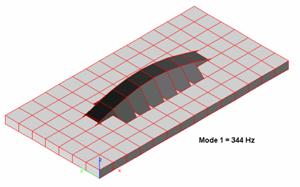
Here are the results, in graphical form, illustrating the magnitude of peak panel displacement at various mode numbers. The panel displacement, as modeled for each simulation series, is exaggerated in appearance for the sake of visual clarity.

Its clear from this model that rectangular panels do exhibit resonance modes, each with a distinct pattern of panel deformation. Indeed, note that different sections of the panel can, at the same moment in time, be moving in opposite directions.

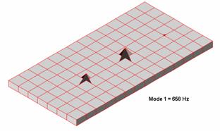
In general, the higher modes will get different areas of the panel moving in opposite directions, effectively diminishing the net acoustic radiation of the panel owing to the diminished net panel area capable of producing the acoustic radiation in the first place. In other words, phase cancellation, arising from different panel areas moving in opposite directions, limits the net amount of total acoustic radiation emitted. Adding to this the fact that higher order modes are easier to damp and we see these self-same modes are generally not in a position to affect system response to the degree the lower order modes are capable of.

For mid-bass cabinets such as the one I'm using here for simulation purposes, I try to shift - as best practices dictates - as much of the resonance series above the system's low pass cut-off point, with the net result, of course, being a quieter cabinet and lower system mechanical noise floor. Let's run some FEA simulations to look at the effects of panel cross-bracing.

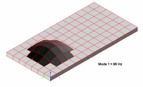
I re-ran the above simulation, this time modeling a series of bracing techniques. For the first simulation, I braced the panel vertically (across the mid-section of the panel. parallel to the front-edge Y-axis, with the following results:

Bracing the panel vertically produced a series of modes clustered around 96 Hz. This upward-shift of the fundamental resonance is a step in the right direction, but not nearly high enough for our purposes.

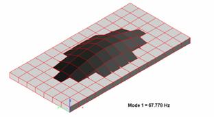
I then modeled the panel braced horizontally, with the brace located at .5y, parallel to the x-axis and running the full length of the panel.

The following results were produced:

In this simulation, the upward shift of the natural panel resonance frequencies is quite apparent, producing superior results to that of the vertically-positioned brace. For a cabinet to be used for the reproduction of the mid-bass portion of the total system response, this is again a step in the right direction, but still not high enough for our purposes.

In actual practice I use multiple horizontal braces for a mid-bass system of this size. Modeling two braces located approximately one third and two thirds up the y-axis (front) edge of the panel and running to the back edge of the panel produces the following results:

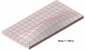
The frequency at which the fundamental natural panel resonance occurs is certainly closer to 430 Hz but I'd like to see the mode series pushed higher. Modeling 3 braces, placed at .25y, .5y, and .75y and running the full length of the panel from front to back produces the following results:

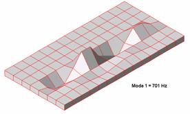
The first mode of vibration is now above the low-pass cut off frequency, but only by about a half octave. I could add another brace, which would certainly push the mode series higher. Since we already know, by virtue of the preceding simulations, that bracing works well, I chose at this point in the series to instead to re-run the simulation, keeping the 3 braces in place, but now doubling the thickness of the panel to 38mm (1.5"). Doing so produced a 1st mode resonance frequency of 701 Hz.

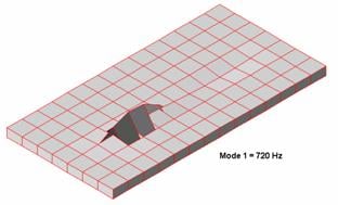
Not bad. Doubling the pane thickness again produced the following results:

Here we see the fundamental mode frequency increase a bit to 720 Hz. There are, of course, practical limits to how much bracing one can employ or how thick panel walls can be made in a design. There's also a diminishing returns effect in place that constrains a designer as to how far one can reasonably expect to go with increasing the amount and type of bracing or how thick the panel walls can be made.

Lowering Mechanical Noise Floor in Speakers - page 2

The Mathematics

The classic equation for determining the resonance frequencies of a uniform, isotropic, rectangular panel, with boundary conditions set as all edges, simply supported (ss) is:

 

 

 

and for the same panel with boundary conditions set as all edges clamped (c), the fundamental resonance frequency can be found with:

 

 

Where:

 

 

Resonance frequency, Hz

D = , flexural rigidity or bending stiffness of plate

m, n = mode numbers, integers

ρ = panel mass per unit area

E = Young's modulus, modulus of elasticity

h = panel thickness

a = panel length

b = panel width

ν = Poisson's ratio (ratio of orthogonal straining)

 

A few caveats are in order where it comes to these equations. First, note the phrase "isotropic". Isotropic means a material that exhibits mechanical properties (such as Young's modulus) that are independent of which direction the measurements are taken from which the mechanical properties are calculated. A good example of an isotropic material would be MDF or, as mentioned previously, a polymer composite material.

 

A material such as plywood would not be considered isotropic, but rather orthotropic, which means it's measured mechanical properties are dependent on the direction (laterally, transversely or radially) being considered.

 

A second caveat is in order: when you start cutting openings in the panel, the formulae are no longer applicable and measured versus calculated resonance values will differ substantially. This doesn't mean the formulae aren't useful in speaker building, they are. But I would use them only as a starting point for working up a rough estimate of panel resonance frequency for those panels that don't have openings cut into them and only if I were using an isotropic material such as MDF or a polymer composite.

 

As mentioned earlier, the contribution to total system acoustic output made by the panels making up a loudspeaker cabinet does not arise solely from the mechanical vibrations set up in each panel by the motion of the driver's frame and other adjacent panels. Another factor, the outward transmission by the outer side of a panel due to fluctuating pressure incident to the internal side of a cabinet panel needs to be considered. For following analysis, it is again assumed the panels behave as plates, clamped at each edge and under uniform load by the driver diaphragm-induced acoustic pressure fluctuations.

 

In any case, the internal pressure fluctuations found within a loudspeaker cabinet under normal operating conditions aren't very large to begin with and further decrease as frequency increases. The internal box pressure created by an operational driver bolted in to one panel of the cabinet can be found, to a good first approximation, by:

 

 

 

Where:

 

 

 

Pb = Rms box pressure, Pascals

Pa = radiated acoustic power, Watts

c = velocity of sound in air, ~345 m/s

ρ o = density of air, 1.18 kg/m^3

Vb = net internal box volume, Liters

f = frequency, Hz

 

 

 

 

Running a series of simulations, holding Pa constant at .1W and varying Vb, using the above equation well illustrates this:

 

 

One commonly seen mathematical method used for expressing the degree to which a panel can reduce the outward expression of these internal pressure fluctuations is by transmission loss.

 

Transmission loss, in dB, is expressed mathematically by:

 

Where τ , the transmission loss coefficient, is expressed by:

 

 

incident pressure

transmitted pressure

 

 

 

Factoring in panel mass and frequency, the TL equation then becomes:

 

 

Where:

 

 

m = panel surface density, ( ρ * h)

ρ = material density

h = panel thickness

ω = radian frequency

z = panel material impedance

 

 

 

 

Taking into account m, and solving for B, the bulk modulus or effective stiffness of the panel is found by:

 

 

 

And from the results of the preceding equation we can now calculate the panel's critical frequency:

 

 

 

Finally, we can finally calculate, the transmission loss slope below /2:

 

 

And the slope above :

 

 

Lowering Mechanical Noise Floor in Speakers - page 3

Once the TL values have been calculated, assessing the effective reduction of transiting acoustical energy by the panel becomes a simple matter of subtracting TL from the dB SPL level of the source, in this case, those levels obtaining in the immediate vicinity of the cabinet-internal side of the panel.

These expressions are, of course, panel-focused and the majority of transmission loss theory found in the literature - upon which these equations are based - is for wall-sized (or larger) "panels" dividing room-sized "enclosures" sporting ideal (or completely lacking) boundary conditions. The results are not necessarily applicable to panels of the material type, dimensions and boundary conditions commonly found obtaining in loudspeaker enclosures.

A search for a better enclosure-focused approach to characterizing the outward re-radiation of acoustic energy by an enclosure's panels brings us to the concept of insertion loss. Mathematically, the general expression of insertion loss (IL) is defined as:

Where:

= acoustic sound pressure level, external to cabinet panel

= acoustic sound pressure level, internal to cabinet panel

The equation is instructive but nevertheless descriptive in nature.

Fortunately, there exists a predictive mathematical expression for determining the insertion loss of a loudspeaker cabinet panel that takes in to account various factors such as enclosure volume impedance, panel mechanical impedance and so forth. For a close fitting cabinet (one where the distance from internal sound source to any panel is 1m or less), with clamped boundary conditions obtaining, IL can be mathematically stated by:

Where:

k = acoustic wave number,

λ = wavelength

d = distance from source to panel

density of air

c = speed of sound in air

and

Where:

a = panel length

b = panel width

h = panel thickness

ρ = density of panel material

ω = frequency of interest

and

which is the complex bulk modulus of the panel material

η = internal damping coefficient of the panel material

E = Young's modulus or modulus of elasticity

ν = Poisson's ratio (ratio of orthogonal straining)

For a polymer composite panel with the material properties as listed in the above table and with the dimensions: a = 20" (.508 m), b = 10" (.254 m), and h = .75" (.01905 m) we can calculate , K and finally IL.

Graphing IL we get:

Here we see a series of nulls alternating between peaks in IL values. Clearly, the response of a cabinet's panels are dependent on both the frequency of the various excited modes and the frequency generated by the driver enclosed within the cabinet; the IL response at higher frequencies is controlled by various material properties along with the distance between the panel and driver.

When panel vibration is in phase with the incident pressure wave, the panel becomes acoustically "invisible" to the incident pressure wave. Standing waves within the enclosure, having the characteristic values of:

, ,

and frequencies that can be approximated by:

Where:

c = speed of sound in air,

nx, ny, nz = 0, 1, 2, 3 …

lx, ly, lz = internal length, width depth

can produce acoustic wave pressures greater than that generated by the driver itself. This can result in panel vibration of a magnitude sufficient to be considered a sort of negative insertion loss.

Curious to see how varying the values of various parameters would affect the IL dB levels, I ran a detailed series of simulations.

First I varied panel length.

Then I varied panel width

Varying length and width, individually, did indeed alter the IL response spectrum. I then varied a and b, simultaneously. In all three cases, as the panel became smaller we see an increase in the frequency of the first null as well as an increase in IL

I then varied panel density. Across the IL response spectrum we see that increasing density increased the amount of insertion loss. All else being equal, we can thus expect that the denser a given panel's material, the quieter it will be.

Then, I varied panel thickness. Increasing panel thickness increases effective stiffness, which results in increased insertion loss, particularly noticeable at the lower end of the IL response spectrum, where insertion loss is controlled directly by the panel's effective stiffness.

Lowering Mechanical Noise Floor in Speakers - page 4

Lastly, I varied the panel material's Young's modulus, a mechanical parameter that effectively characterizes a panel's stiffness. As expected, we see that IL response variations happen primarily in the lowest decades of the IL response spectrum; IL increases as E increases. Note too that with increased stiffness we see the first, lowest frequency IL minimum shift upward in frequency.

To complete the simulation run, I applied various simulated IL response spectra to actual db-SPL driver response curves, which resulted in predicted panel acoustic response, when driven by the acoustic pressure waves generated by the driver enclosed within the simulated polymer composite cabinet. The simulations were then run, producing predicted results of dB-SPL measurements, taken at 1 meter, outside the cabinet.

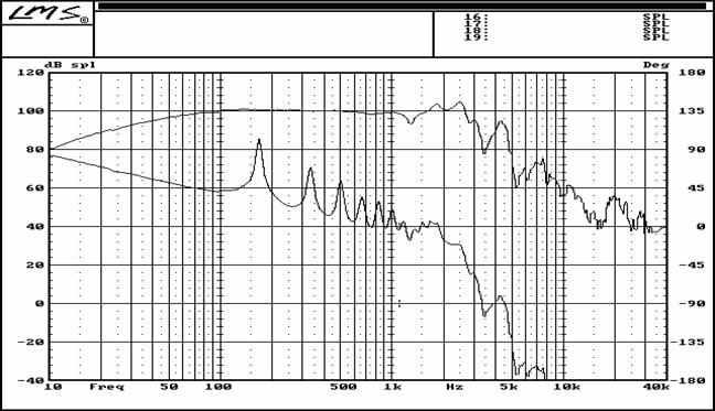
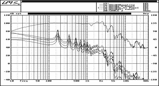
Baseline

The top curve is the dB-SPL response of the driver, measured at one meter. The bottom curve is that of the predicted response as measured at a distance of 1 meter outside the simulated cabinet that totally encloses the driver.

Keep in mind these results are for an enclosure that contains no sort of sound-absorbing filling or liner; thus the thermodynamic condition obtaining within the enclosure is adiabatic. As well, the simulation does not take into account panel acoustic output resulting as a consequence of mechanical vibrations originating at the driver's frame.

At any rate, once having established a performance baseline I then ran a further set of simulations, each with the purpose of exploring the effects of varying mechanical properties of the cabinet panel's material. (Keep in mind that in each of the following simulations the top curve hovering around 100 dB Spl is that of the driver when not enclosed by the cabinet.)

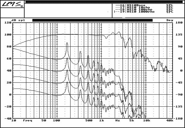
Density Variations

My first simulation series held all properties constant, except for density. Varying density produced substantial differences in the amount of insertion loss and in turn substantial affects on panel acoustic output. The resulting curves show that more dense the material, the higher the insertion loss, resulting in a decreased panel dB SPL levels.

Next, I re-ran the simulation, this time holding all parameters constant, save stiffness. Increasing stiffness did

have an effect on IL, but it took quite a substantial increase in panel stiffness before significant changes

in IL and thus panel acoustic output became evident. We can see from the graph that IL did increase as stiffness increased, and at the lower end of the response spectrum, just as predicted by theory.

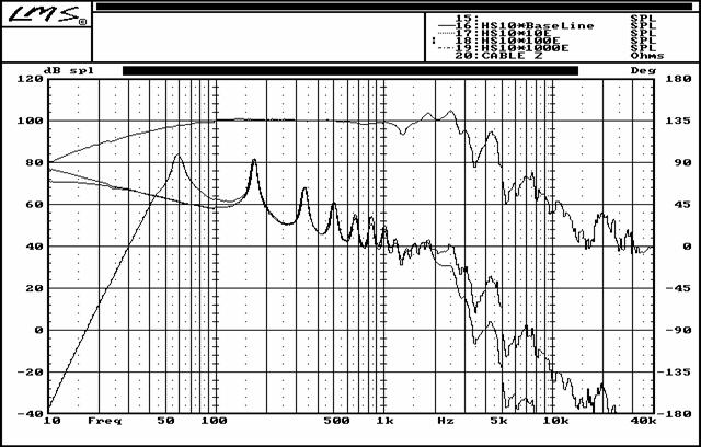
Stiffness Variations

Last, I ran a series of simulations holding all parameters constant, save thickness. As we can see in the accompanying graph, increasing panel thickness increases IL.

Conclusion

In this article we have seen that panel resonances, either structural or airborne in origin, can have effects, usually deleterious in nature, on system response. We have also seen that the designer has at his or her disposal a effective means by which these resonances can be damped, dispersed or otherwise shifted out of the frequency range of interest. I think it also fair to say that the use of such modeling techniques as FEA can be an invaluable, efficient tool where it comes to exploring various design solutions when seeking to lower the mechanical noise floor of the system.