
Dayton Audio WT3 Woofer Tester Review
- Product Name: Dayton Audio WT3 Woofer Tester
- Manufacturer: Dayton Audio
- Performance Rating:


- Value Rating:
- Review Date: April 17, 2008 18:50
- MSRP: $ 99.88US.unit
Primary Use: Woofer impedance measurement, Thiele/Small
parameter generation
Secondary Use: Impedance measurement of drivers other than
woofers and a variety of passive components.
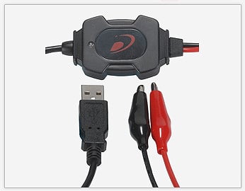
System Type: USB (USB 1.1 compliant, USB 2.0, preferred).
Connector: 1 pair, built-in alligator clips
Power requirement: Unit draws power from USB port; no
batteries or external power supply
required.
Test signal: Upward-swept Sine wave
Frequency Display/Sweep Width (Hz): Adjustable LF & HF points
LF Limits: 1 Hz to 10 kHz
HF Limits: 10 Hz to 20 kHz
Software: Program included, must be installed manually
Calibration resistor supplied
Hardware manufactured in China,
software in USA.
Warranty: Warranted free from defects in material and
workmanship for 5
years from date of purchase .
Pros
- Easy to install & easy to use
- Impressively accurate measurement data
Cons
- Quirky user interface
- Limited data post-processing capabilities
- Minimal help section & user manual
Introduction
 Today’s loudspeaker
DIYer is fortunate in having quite a few choices to select from when it comes
time to choosing the measurement tool (or tools) needed to achieve a successful
project outcome. Critical to the project’s design process is being able to
accurately assess the Thiele/Small driver parameters of the various mid-range,
woofer and subwoofer drivers being considered. (Tweeters are typically handled differently, though accurate tweeter
impedance & amplitude response data are just as essential to the
design process as it is for all other drivers used in the system).
Today’s loudspeaker
DIYer is fortunate in having quite a few choices to select from when it comes
time to choosing the measurement tool (or tools) needed to achieve a successful
project outcome. Critical to the project’s design process is being able to
accurately assess the Thiele/Small driver parameters of the various mid-range,
woofer and subwoofer drivers being considered. (Tweeters are typically handled differently, though accurate tweeter
impedance & amplitude response data are just as essential to the
design process as it is for all other drivers used in the system).
If the budget doesn’t leave room for the pricier measurement tools out there or you’d simply rather spend more on the hardware you pack your cabinets with than on the gear you measure it all with, then Dayton Audio’s WT3 Woofer Tester may be the perfect choice for the job. Its inexpensive, easy to install and use and the accuracy of the data produced can rival that of measurement tools costing 10x as much or more!
First Impressions
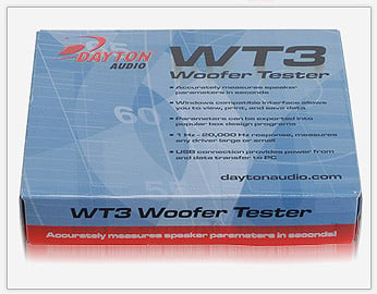 Everything comes packed in a smallish box and the kit
includes the hardware, a hardcopy, single page quick-start quide, the
installation CD and a calibration resistor.
Everything comes packed in a smallish box and the kit
includes the hardware, a hardcopy, single page quick-start quide, the
installation CD and a calibration resistor.
The front page of quick-start guide contains all the information needed to get the software & hardware installed, the system calibrated and also includes basic measurement instructions. The back page of the guide contains extra information for those who’d like to use the WT3 system on PCs running Microsoft Vista.
Setup
 The software installation doesn’t run automatically (as is
typical these days) off of an autorun file: there isn’t one to be found on the CD and the installation won’t
start automatically when you pop the CD in the drive. Rather, you have to
manually hunt for the setup.exe file and run the installation from that. (Partially in response to this review Dayton
Audio will be adding an Autorun.inf file to the WT3 distribution CD so that
installation will begin automatically when the CD is inserted). As well,the limited
Help Topics section mentioned at the top of this review are currently
being expanded to better cover impedance measurements of resistors, inductors,
closed and vented boxes.
The software installation doesn’t run automatically (as is
typical these days) off of an autorun file: there isn’t one to be found on the CD and the installation won’t
start automatically when you pop the CD in the drive. Rather, you have to
manually hunt for the setup.exe file and run the installation from that. (Partially in response to this review Dayton
Audio will be adding an Autorun.inf file to the WT3 distribution CD so that
installation will begin automatically when the CD is inserted). As well,the limited
Help Topics section mentioned at the top of this review are currently
being expanded to better cover impedance measurements of resistors, inductors,
closed and vented boxes.
Once installed, however, everything needed to run the WT3 system is in place, including the USB Audio Codec.
Overall, the installation of the WT3 compared to that of other commonly available products was quick and easy. The fact that the system is USB-based makes connection quite convenient as well. Overall, once installed, the convenience and ease-of-use of the product in practice is outstanding.
Calibration & Measurement
Once the software is installed, the application is up & running and the WT3 probe is plugged into a USB port everything is in place to finally begin measurement. Two things you’ll notice right away when you do connect the probe to a USB port: a blue LED on the probe lights up and the USB Audio Codec takes over. The blue LED is a minor but nice feature that lets you know the probe is active.
You’ll know the USB audio Codec is active because when it takes control, the PC focuses solely on the WT3 probe to the exclusion of all other audio process, which means you won’t be able, for example, to play music through your PC’s sound card while making measurements using the WT3.
Once the probe is plugged in, the manual recommends a 90-second wait time before you begin measurement. According to the manual, this wait is essential to allow the probe’s circuitry to stabilize. This required start up wait-time is a good time to set the Windows mixer Master Out and Wave levels to max as, once again, recommended by the manual. Setting levels anything above 50% is worth experimenting with; anything below 10% produces noisy, essentially useless data. For this review all measurements were made with Master & Wave levels set at 100%.
 If you need to keep track of your Windows mixer settings for
different audio-related items, use something like Quickmix to keep track of
those settings. Quickmix uses templates you create to keep track of mixer
settings for different applications/requirements. So, for example, if you’re
using your sound card to make dB SPL measurements using software that requires
mixer settings be the same whenever the software is running, you can set up
QuickMix to remember those settings. You can then build a second template to
take care of the settings WT3 needs to see and recall them, via QuickMix,
whenever you need them. It’s a great way to go if you regularly need to recall
different mixer settings for different applications.
If you need to keep track of your Windows mixer settings for
different audio-related items, use something like Quickmix to keep track of
those settings. Quickmix uses templates you create to keep track of mixer
settings for different applications/requirements. So, for example, if you’re
using your sound card to make dB SPL measurements using software that requires
mixer settings be the same whenever the software is running, you can set up
QuickMix to remember those settings. You can then build a second template to
take care of the settings WT3 needs to see and recall them, via QuickMix,
whenever you need them. It’s a great way to go if you regularly need to recall
different mixer settings for different applications.
At any rate, once the probe is plugged in, the software up & running and the appropriate levels set in the mixer, its time to calibrate. Calibration of the WT3 involves both calibrating out the impedance of the probe leads as well as calibrating the system to the supplied 1 kΩ, 1% resistor. If you have a way of accurately measuring the value of the calibration resistor, then by all means do so and use that value when you run the Impedance Calibration utility. In the case of the calibration resistor supplied with this review sample, the actual value measured was .9976 kΩ. (Note: the measured value of the calibration resistor should only be used if the meter’s accuracy is BETTER than 1% (the resistor’s rating).
Both calibrations are easy enough and each takes just a few seconds to run. Click on Impedance Analyzer…, then Test Leads Calibration…, connect the WT3’s alligator clips together and run the calibration. Once that’s done, connect the supplied 1 kΩ calibration resistor to the alligator clips. Click on Impedance Analyzer… again, then Impedance Calibration … You’ll then be presented with a screen that asks for the value of the calibration resistor. Enter that value and click OK, the system calibrates itself and you are now ready to begin actual measurement.
Running both calibrations prior to actual measurement is essential to ensuring the measurement data you’ll be generating is as accurate as possible.
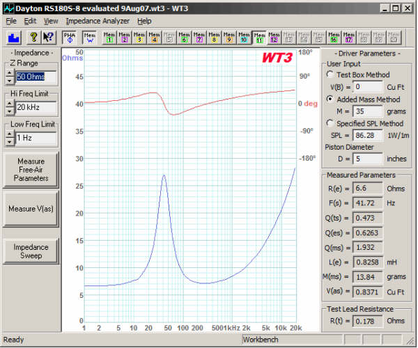
WT3 Measurements and Analysis
I. Driver Impedance
So how accurate is this thing? How does it compare to other measurement tools out there, in terms of accuracy? What features does it have? To answer these and other questions, let’s look at how the WT3 stacks up against LinearX’s LMS system. Some back-to-back measurement comparisons are in order.
Impedance plots of a 10” Woofer, 4” midrange and 1” concave-domed tweeter were made using the WT3 and LinearX’s LMS system. The results for each driver are shown below in the left hand column. In each case, the blue plot is the LMS data and the red plot is the WT3 data. To further aid in comparison, the WT3 plots were normalized to the LMS plots. The results are shown in the right hand graphics column.
Figure 1a & b. At left: Tweeter free-air impedance, Mag. & Phase. At right, WT3 data normalized to LMS data.
Figure 2a & b. At left: Midrange free-air impedance, Mag. & Phase. At right, WT3 data normalized to LMS data.
Figure 3a & b. At left: Woofer free-air impedance, Mag. & Phase. At right, WT3 data normalized to LMS data.
II. Thiele/Small Driver Parameter Derivation
Aside from its ability to capture impedance measurement data, the most important feature of the WT3
is its ability to derive a driver’s Thiele/Small parameters from the impedance plots.
Basically, the process runs as follows: (1) the free-air impedance of the driver under test is measured; and (2) the delta-mass, delta-compliance impedance plots are generated or specified db spl method is used. The raw measurement data is then processed by WT3, mathematically deriving the required Thiele/Small parameters. With those parameters at hand, a suitable cabinet design can then be worked up.
To further put the WT3 to the test, two enclosures were designed and the amplitude response & impedance plots were modeled for comparison purposes. One design is based on the Thiele/Small parameters as generated by LMS data and the other based on the same parameters generated by WT3 data. Below is a table of the Woofer’s Thiele/Small parameters as derived from the two systems measurements.
| WT3 |
LMS |
| Revc = 7.059 Ohm | Revc = 7.06 Ohm |
| Fo = 43.9 Hz | Fo = 44.48 Hz |
| Sd = 349.00 cm² | Sd = 349.00 cm² |
| Vas = 40.04 ltr | Vas = 42.03 ltr |
| Mms = 56.8 g | Mms = 52.701 g |
| Qms = 5.42 | Qms = 6.42 |
| Qes = 0.806 | Qes = 0.782 |
| Qts = 0.702 | Qts = 0.697 |
| SPLo = 88.11 dB | SPLo = 88.621 dB |
Modeling a sealed, high-pass enclosure (Butterworth alignment) with a Ql = 2, produced a cabinet with a net internal of 1.66 ft^3 (46.95 ltrs) for the WT3 data and a cabinet with a net internal volume of 1.70 ft^3 (48.2 ltrs) for the LMS data, an enclosed volume difference of just under 3.0%. Showing above are the amplitude response plots (left) and impedance plots (right) of the 2 systems modeled. Purple plots are for the system based on LMS data and green for the WT3 data.
Though the parameters are generally in good agreement, there are differences. Taking into account differing drive conditions and different post-processing algorithms in each of the products helps to keep these differences in proper perspective. All in all, not bad for a product that costs less than 1/10th the price of the LMS system!
III. Passive Component Impedance Measurement
Another handy feature is the WT3’s ability to measure the impedance of various electrical components, such as the caps, resistors, and inductors found in the passive crossovers commonly used in loudspeaker systems. It should be noted in passing that the WT3 is not officially specified for measuring capacitors, though it did a pretty good job of it, nonetheless
A good deal of useful information can be derived from a components impedance plot, including the actual resistance, capacitance and inductance values at a specified frequency (especially useful information when working up loudspeaker crossover network designs). Let’s compare the WT3 and LMS performance in measuring the impedance of some component samples.
Above are (from left to right) impedance plots for a resistor, inductor and capacitor. In each case the blue plots are generated by WT3 and the green plots by LMS.
For the resistor, the WT3 has accurately measured the component’s value (as confirmed by an HP 3455A Digital VOM) across the entire measurement frequency spectrum. (The odd jumps seen in the green plot at 100, 1k & 10k are systemic measurement artifacts generated by LMS; the WT3 did not present any such glitches and overall presented a cleaner, more accurate plot of the test resistor’s impedance.
For the inductor, the LMS and WT3 impedance values across the frequency spectrum agreed to within a fraction of an ohm.
The capacitors impedance values were in good agreement across the 1 kHz – 10 kHz portion of the spectrum, with the values diverging outside the band. (The shelving seen below 100 Hz in the LMS plot is a direct result of LMS system impedance measurement limit set to 1 kHz). Not bad for a product not specified for capacitor measurement!
Odds & Ends
The Dayton Audio’s WT3 is product designed to measure impedance only. It will not make dB spl measurements of the driver/system under test. For that you’ll need to rely on some other measurement software/system. You’ll also need to look elsewhere to model system simulations based on the raw data/T/S parameters generated by WT3. Fortunately, the WT3 application includes an export utility that makes it easy to do all your post-processing/simulation work outside the program. (There’s an import utility as well). For the job it is designed to do, the WT3 does very well indeed.
The few quirks found in the review sample mainly relate to the user interface. For example, the Ctrl-V (Paste) keystroke sequence wouldn’t paste text data into text boxes ordinarily used for data entry. Also, the text box used in the Impedance Calibration screen is masked in such a way that you can’t enter a value such as “.9967”; rather it needs to see “0.9967”.
Additionally, there is no mouse (or other) cursor function
attached to the measurement plots; you can’t use a cursor to scroll across the
plots to look at individual datapoint values. To view individual datapoint
values, you’d need to export the raw data as a text file and read the
information from the resultant file.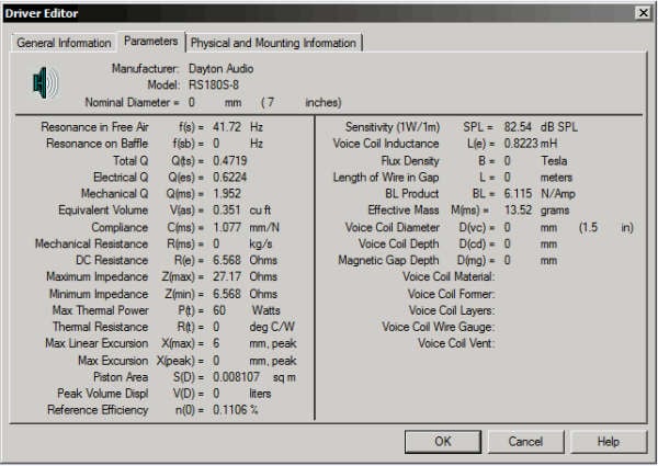
The WT3 allows you to save up to 20 impedance plots in memory, though it provides no direct way to name them. This isn’t an issue if you’re working with only 2 plots. But if you’re working with 20 plots, how long before you forget just exactly what plot # 7 is? (WT3 does allow collections of saved impedance plots to be saved as a Project file). To be fair, it should be mentioned you can save 3 tabbed pages worth of text data per driver measured (the Workbench Measured parameters are filled in automatically as measurements are taken), using the handy Driver Editor utility, shown at right.
Conclusion
Dayton Audio’s WT3 Woofer Tester is a budget-priced measurement tool for working up impedance plots of raw drivers and various electrical components, such as resistors, caps and inductors. It can also provide the all-important Thiele/Small parameters, essential to the loudspeaker design process.
The product is easy to install and easy to use. Though purposely limited in its capabilities, what it does do it does very well, in a number of important ways comparing favorably to a system costing better than 10 times as much. Not bad!
Dayton Audio WT3 Woofer
Tester
MSRP: $99.88US/unit
http://www.daytonaudio.com
The Score Card
The scoring below is based on each piece of equipment doing the duty it is designed for. The numbers are weighed heavily with respect to the individual cost of each unit, thus giving a rating roughly equal to:
Performance × Price Factor/Value = Rating
Audioholics.com note: The ratings indicated below are based on subjective listening and objective testing of the product in question. The rating scale is based on performance/value ratio. If you notice better performing products in future reviews that have lower numbers in certain areas, be aware that the value factor is most likely the culprit. Other Audioholics reviewers may rate products solely based on performance, and each reviewer has his/her own system for ratings.
Audioholics Rating Scale
 — Excellent
- — Very Good
- — Good
- — Fair
- — Poor
| Metric | Rating |
|---|---|
| Build Quality | |
| Appearance | |
| Performance | |
| Value |