
Bi-Wiring A Loudspeaker: Does it Make a Difference?
Biwire Waveform
Originally published at: University of St. Andrews, St Andrews, Fife KY16 9SS, Scotland.
“Bi-wiring” is a controversial topic. Some people are quite certain it
makes an audible difference. Some others are convinced that it can’t
actually make any difference at all. The purpose of this analysis is to
try and decide whether it is at least theoretically feasible that
bi-wiring can make any difference.
To define what is meant by “bi-wiring”, and understand what effects it
may (or may not) have, we can start by considering the situation
illustrated in Figure 1.
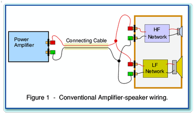
This shows an amplifier connected to a loudspeaker by a
standard cable made from a pair of connecting wires. For clarity, only
one channel of a stereo pair is shown. The loudspeaker consists of two
drive units. – a high-frequency (HF) unit often called a “tweeter”, and
a low frequency (LF) unit often called a “woofer”. Loudspeakers
generally employ a “cross-over network” to direct low signal
frequencies to the woofer, and high frequencies to the tweeter. In the
example shown here this network is split into distinct HF and LF
sections. This split permits the loudspeaker to be bi-wired. (Not all
loudspeaker cross-over arrangements will permit this without
modification.) In practice, as shown here, loudspeakers designed to
permit bi-wiring have extra sets of input terminals which may be joined
together when bi-wiring is not employed.
In the conventional wiring arrangement shown in Figure 1, the
HF and LF input terminals are wired together in parallel at the
speaker, and just one pair of connecting wires are employed to link
both speaker units to the amplifier. In most cases “bi-wiring” means
using an extra pair of connecting wires (i.e. another cable) so that
the signals for the tweeter and woofer are sent from the amplifier to
the speaker by separate routes. This bi-wiring arrangement is
illustrated in Figure 2. In this new arrangement, Cable 1 carries the
signals destined for the tweeter, and Cable 2 carries the signals
destined for the woofer.
Various arguments have been presented for this bi-wiring arrangement by adherents who feel it alters the sound. For example, it may be claimed that each of the two cables may now be optimised in some way for the limited range of signal frequencies it now carries, and hence act more effectively. Alternatively, it is sometimes claimed that separating the signals for the tweeter and woofer means they do not now ‘interfere’ in some manner which may arise when they share the same cable. Unfortunately, these claims are generally unclear in technical terms, and there is a general lack of any reliable analysis or measured data to support the claims. This makes it questionable whether the claims are justified. It is also unclear whether the alternative arrangement in Figure 3 might also be “better” than the conventional arrangement. The arrangement in Figure 3 is also bi-wired, but the pairs of wires are now joined at both ends of the signal connection from amplifier to loudspeaker.
In the modified arrangement shown in Figure 3 both
cables are used “in parallel” to connect signals to both speaker units.
The question now becomes, “Are the arrangements shown in Figures 1, 2,
and 3, all going to produce exactly the same results in use?”
Detailed analysis of the three arrangements is made difficult
by two factors. Firstly, the electrical properties of the items
involved can be quite complicated. The networks used in loudspeaker
crossovers may contain a number of components and have a complex
behaviour. Similarly for the actual speaker units. As we have seen on
the webpages on cables, even the behaviour of simple twin-feed
connecting cable can be more complicated that we might expect.
The second problem for a precise analysis is that the actual
details of the loudspeaker crossover, etc, will vary a great deal from
one model of loudspeaker to another. Hence we can expect any results to
depend upon the choice of loudspeaker, cable, etc.
To make understanding these questions easier we can address a
simpler question – i.e. we can ask, “Is is possible for the changes
between the arrangements in Figures 1 - 3 to make any difference, or
not?” To answer this question we need only look at a simplified
example. If, in that example, a difference can be show to be possible,
then it implies that a difference may appear even in more complicated
arrangements. If no such difference is shown, this does not necessarily
resolve the real issue, but at least we have progressed part of the way
to a better understanding. With the above in mind we can now form a
electronic models of the above arrangements, simplify them as far as
seems reasonable, then compare their computed behaviours.
Bi-Wiring A Simple Model
Before analysing the (possible) effects of bi-wiring we need to
establish a suitable simplified model of the loudspeaker. One of the
simplest possible arrangements is illustrated in Figure 4.
In this model the cross-over (filter) networks are deliberately assumed to be about as simple as possible. A series inductor,  , is uses to prevent high frequencies from reaching the woofer, and a series capacitor,
  , is used to prevent low frequencies from reaching the tweeter. Each actual loudspeaker unit is regarded purely as an effective Radiation Resistance value,
  and
and  .
The acoustic power radiated by each unit is then assumed to be
proportional to the square of the current through its radiation
resistance value. (i.e. the sound pressure produced by each is assumed
to be proportional to the current.)
.
The acoustic power radiated by each unit is then assumed to be
proportional to the square of the current through its radiation
resistance value. (i.e. the sound pressure produced by each is assumed
to be proportional to the current.)
In reality, any practical speaker will have much more complicated properties. However since we are only concerned with seeing if it is possible for bi-wiring to make a change, we can use a simple model of this type. It is, however, important to bear in mind that this means we must interpret any results of our analysis with caution. This is because – even if we conclude that a change may occur – our results cannot be taken as a guide to what level or form such changes may take in a more realistic situation. Hence we are only addressing the “in principle” question of seeing if a change might arise due to bi-wiring. A more detailed and case-specific analysis would be required to assess whether any changes which might arise in a given case were of any audible significance.
For convenience we can assume that  , where
  is a conveniently chosen standard resistance value. Each of the
crossover/unit combinations will have a turn-over frequency set by the
chosen values. This will determine the frequency range within which
each part of the loudspeaker is responsible for ensuring signals are
audible. Again, for simplicity and convenience we can assume these have
been set to both equal the same value,
is a conveniently chosen standard resistance value. Each of the
crossover/unit combinations will have a turn-over frequency set by the
chosen values. This will determine the frequency range within which
each part of the loudspeaker is responsible for ensuring signals are
audible. Again, for simplicity and convenience we can assume these have
been set to both equal the same value,  . Hence we can say that

The input impedance ,  of the tweeter, and the input impedance,
  of the woofer will therefore be

Before considering the effects of amplifier-speaker cabling we can now determine the inherent properties of the loudspeaker. Firstly, when its units are used in parallel (as in Fig 1) we can say that the loudspeaker’s impedance will be

where  represents the parallel combination of the two values.
In this specific, simplified, case it turns out that when we calculate  it equals
  at all frequencies. This result will, of course, not be true in
general, so we must interpret any results based upon this particular
speaker model with care.
at all frequencies. This result will, of course, not be true in
general, so we must interpret any results based upon this particular
speaker model with care.
In terms of acoustic output we may say that the pressure radiated by
each speaker unit will vary in proportion with the current at each
instant through its radiation resistance. We may represent the current
through the tweeter as  and that through the woofer as
  .
Since the radiation will add coherently we may say that the total sound
pressure created will be proportional to the vector total current,
.
Since the radiation will add coherently we may say that the total sound
pressure created will be proportional to the vector total current,  . The mean power will therefore be proportional to
  , and any phase changes will depend upon the relative phase of the driving signal and the total current.
When using the loudspeaker modelled here we can now represent the situation when employing a single cable (i.e. not bi-wired) by the circuit shown in Figure 5.
Here we can represent the output impedance of the power amplifier as a series impedance,  , and the impedance of the cable by
  . Note that
  does not represent the characteristic impedance of the cable as a
transmission line. It is simply the series resistance and/or inductance
of the cables being used.
does not represent the characteristic impedance of the cable as a
transmission line. It is simply the series resistance and/or inductance
of the cables being used.
When the amplifier asserts an output (a.c.) voltage of  this will result in a voltage,
  ,
appearing at the loudspeaker terminals. In this simple case we know our
loudspeaker has an input impedance (tweeter and woofer sections linked
in parallel) of
,
appearing at the loudspeaker terminals. In this simple case we know our
loudspeaker has an input impedance (tweeter and woofer sections linked
in parallel) of  . Hence we can say that

In situations where the cable and amplifier impedances
are frequency dependent (and not simply resistive) this will lead to a
frequency-dependent degree of attenuation, and some relative phase
dispersion. However if  and
and  are substantially resistive and independent of frequency the main
result is a small reduction in the volume of the resulting sounds. The
total load seen by the amplifier will be
are substantially resistive and independent of frequency the main
result is a small reduction in the volume of the resulting sounds. The
total load seen by the amplifier will be  at all frequencies in this situation. Hence the power efficiency of the system at all frequencies will be proportional to
  .
.
The circuit is a fairly simple one and has only one current node. This means we can immediately say that

where  is the current being produced by the amplifier at any instant.
The situation when using a bi-wiring arrangement may be represented by
the circuit shown in Figure 6. For simplicity it is assumed that the
two cables are identical.
As with the previous case, if we assume the cable impedances are essentially resistive then their effect is to increase the total resistance seen in the high-frequency and low-frequency ‘arms’ of the circuit by the same amount. At first sight this seems to imply that we have essentially just altered the overall load by the same amount as before. However this may not be the case as the presence of the separate cable impedances will independently affect the nominal turn-over frequencies of the low-pass and high-pass networks employed. The special case we initially envisaged was that the turn-over frequencies (as well as the load resistances) of the two arms were identical. This meant their parallel combination was purely resistive. However we may now have ‘unbalanced’ the arrangement so that this is not longer true.
As with the single-cable arrangement, the system illustrated
in Figure 6 has a single node. Hence we can say that the power
efficiency will simply depend upon how  may vary with signal frequency. We may therefore look to see if the
total load impedance now varies with frequency as if it does, this
implies that the above bi-wired arrangement may be expected have a
frequency response that differs from that produced with a single cable.
may vary with signal frequency. We may therefore look to see if the
total load impedance now varies with frequency as if it does, this
implies that the above bi-wired arrangement may be expected have a
frequency response that differs from that produced with a single cable.
Bi-Wiring Examples of Results
To assess the implications of the model of bi-wiring we have produced
we can now examine the results of choosing some example values. For
simplicity, the following assumes that the nominal impedance of the
loudspeaker units is such that  , and that the nominal cross-over frequency is
  kHz. Figure 7 shows the input impedance of the resulting loudspeaker
system as a function of frequency. Note that the frequency scale is
logarithmic, and that in each case it is the magnitude (modulus) of the
impedance that is plotted as a function of frequency.
kHz. Figure 7 shows the input impedance of the resulting loudspeaker
system as a function of frequency. Note that the frequency scale is
logarithmic, and that in each case it is the magnitude (modulus) of the
impedance that is plotted as a function of frequency.
Figure 7 and the graphs that follow have been plotted
from numerical results obtained from some simple C++ programs. The
results shown in Fig 7 confirm that our simple model has the property
that the impedance of the LF and HF sections when used connected in
parallel is equal to  at all frequencies. This may be understood in terms of regarding the
variations in impedance of the LF and HF sections cancelling out.
at all frequencies. This may be understood in terms of regarding the
variations in impedance of the LF and HF sections cancelling out.
Let us now consider using an amplifier whose output impedance
is 0·1 Ohms, and cables whose series resistance is 0·1 Ohms. For
simplicity, we ignore cable inductance and assume that the cable is
essentially purely resistive. We can now compare the results of using a
single cable of this type (arrangement as shown in Fig 5) with using a
pair of identical cables (arrangement as Fig 6). Figure 8 shows the how
the total impedance seen by the amplifier varies with frequency in each
case.
The broken black line in Figure 8 shows the impedance
seen by the amplifier when using a single wire. Since this means the HF
and LF units are connected together in parallel at the speaker end of
the cable, the speaker looks like an 8 Ohm load at all frequencies. The
signal voltages being generated by the amplifier see this impedance
through the series impedance of the amplifier output and cable, thus in
this case producing a total impedance of 8·2 Ohms at all frequencies.
The solid blue line in Figure 8 shows the impedance seen by
the amplifier when bi-wiring is employed. In this case an independent
0·1 Ohms of cable impedance is seen in series with the HF and LF
sections. The parallel combination is then seen in series with the
amplifier’s output impedance. The bi-wiring arrangement can be seen to
modify the impedance of the system as seen by the amplifier in a
frequency dependent manner. The chosen cross-over frequency for this
example was 1 kHz. Looking at Figure 8 it can be seen that changing
from using a single cable to a bi-wiring arrangement caused a change in
overall impedance which is most noticeable at this frequency. In this
case it can be seen that at 1 kHz the total impedance of the system
seen by the amplifier is 0·1 Ohms lower when bi-wired than when a
single cable is employed. This change may be regarded as a consequence
of the separate cable impedances altering the effective roll-over
frequencies of the HF and LF sections so that they are no longer
identical. The result is that the system’s impedance value is no longer
constant over the whole frequency range.
The above result is an interesting one as it implies that
bi-wiring may change the impedance properties of the total load system
seen by the amplifier. If the sound power produced depends upon the
square of the current fed to the system, this implies that the
frequency response may perhaps be changed by bi-wiring as a result of
interactions between the choice of cabling arrangement and the input
impedances/networks of the loudspeaker units.
Figure 9 illustrates some examples of the changes in
frequency response which the alterations in system impedance imply may
produce. The curves are for a series of different choices of cable
series resistance/impedance,  .
In each case the amplifier output impedance is assumed to be 0·1 Ohms.
Hence we can use this set of plots to get an impression of how the
behaviour may vary if we change the cable resistance but use the same
amplifier and speaker in each case. Looking at the plots we can see
that for these specific examples we happen to get a variation in signal
level at the crossover frequency which, in decibels, is approximately
the same as the chosen cable series resistance in Ohms.
.
In each case the amplifier output impedance is assumed to be 0·1 Ohms.
Hence we can use this set of plots to get an impression of how the
behaviour may vary if we change the cable resistance but use the same
amplifier and speaker in each case. Looking at the plots we can see
that for these specific examples we happen to get a variation in signal
level at the crossover frequency which, in decibels, is approximately
the same as the chosen cable series resistance in Ohms.
Figure 10 shows what happens if we keep the cable
resistances fixed at 0·1 Ohms, and vary the output impedance of the
amplifier. As with Figure 9, a set of curves are plotted, but in this
case for  0, 0·1, 0·2, 0·3, 0·4, and 0·5 Ohms. Looking at Figure 10, we can see
that all these plots are very similar. Indeed, they are so close
together on the graph that it is not obvious how many curves are
plotted. Considering Figures 9 and 10 taken together, leads to the
implication that – in terms of comparing bi-wiring with using a single
cable – changing the cable resistance may have an effect, but that
varying the amplifier’s output resistance has little or no effect.
0, 0·1, 0·2, 0·3, 0·4, and 0·5 Ohms. Looking at Figure 10, we can see
that all these plots are very similar. Indeed, they are so close
together on the graph that it is not obvious how many curves are
plotted. Considering Figures 9 and 10 taken together, leads to the
implication that – in terms of comparing bi-wiring with using a single
cable – changing the cable resistance may have an effect, but that
varying the amplifier’s output resistance has little or no effect.
The above results imply that bi-wiring may alter the frequency
response and that, when using a very simple speaker system with an
impedance of around 8 Ohms, this variation may be of the order of 0·1
dB when using cables whose series resistance is around 0·1 Ohms. Thus,
in principle, it seems possible that bi-wiring may alter the system’s
frequency response. The details of any change will then depend upon the
series impedance of the cables, and the impedance properties of the
loudspeaker.
Two things should be kept in mind, however:
-
In general many loudspeaker cables will have a series resistance value well below 0·1 Ohms. Indeed, a low value is advisable to avoid other types of interaction with the loudspeaker input impedance. Thus in practice the actual variations may well be much smaller than those plotted in Figure 9. As a result, it is debatable if any variations in practice will normally be large enough to be audible or to be regarded as being of any real consequence. Moving your head a few centimetres when listening may have a larger effect in many rooms.
-
The model used here is a very simple one. Hence we should really only consider these results as implying that effects can occur in principle. The plots should not be taken to indicate what will actually happen with a more complex and realistic system.
It is also worth bearing in mind that the
detailed analysis carried out here assume coherent addition of the HF
and LF signals. This will be correct for a a listener at a fixed point
when considering direct radiation from the loudspeaker system. The
situation when the diffuse soundfield of the loudspeaker is taken into
account may be more complex. However for this analysis we are simply
interested in an “in principle” answer. Hence we can see this as
another complication which means the actual performance in reality may
well differ from the above results, but that a small change due to
bi-wiring remains possible.
Thus we can conclude that there may be a small effect due to
bi-wiring, but the above tends to imply it may normally be so small as
to have little significance. In order to say more, a detailed model of
specific realistic systems, and/or some precise measurements, would be
required. These might reveal a more noticeable effect in some cases,
but the above taken by itself implies the effects will usually be very
small if low series impedance cables are used. It is also perhaps worth
bearing in mind that - even in a case where any change in frequency
response is large enough to be audible - this does not establish that
the bi-wired arrangement will inevitably then be “better” than using a
single cable. That would depend upon the circumstances of use, and the
preferences of the listener.
Bi-Wiring Modulation Muddle
This page examines an argument I have seen presented as a technical ‘justification’ for claiming that bi-wiring is different to conventional loudspeaker wiring. Specifically because the resistance of conventional wiring is claimed to produce a form of distortion. An example of this argument appears in a web forum thread that starts at:
The Claim
The central points of the argument are summarised in posting 99 of the above thread so I will quote them below. You may wish to visit the forum and examine the thread to put the following in context, but the quote should suffice for the purpose of what follows:
The currents and the resistance are normalized, so the peak woof and tweet currents are 1, and the resistance of the wire is also normalized to 1.
The woof current is the blue line, the diss is (Asquared) I2R, so as you can see, it peaks at 1, and is always positive (real dissipation cannot be negative).
It is your basic sine squared waveform, a direct result of the woof current flowing through a wire by itself. Note that for an ideal load, this is also exactly the same dissipation time profile scaled differently.
The tweet current is the magenta line, called Bsquared. again, I squared R...
With biwiring, the total wire dissipation is of course, the sum of the two, A squared plus B squared, and the load dissipation at the speakers is an exact scale of the wire dissipation.
The yellow line (asq plus b sq) is the summation of the wire loss in biwiring.
Now, consider both signals travelling in one wire, such as monowiring..
The equation is P = I2R, with I = A + B (A+B)2 = A2 + B2 + 2AB. So, subbing A + B for I creates 3 parts of the power dissipation, the third and most interesting component being the 2AB part..
I put that on the graph, that is the brown (I think) color. Note two very important things about the 2AB component...
1. It goes NEGATIVE!! At first blush, that seems impossible..However, look at it's value compared to the yellow line which is the A2 + B2 part....note that if you sum them, they NEVER go negative. In other words, the 2AB component is a modulation of the expected dissipation. So, the monowire dissipation never goes negative..
2. It is a ZERO INTEGRAL power waveform...in other words, what is below zero is exactly the same area as that above zero. Since FFT algorithms cannot spot a zero integral power waveform, it isn't seen.
Think of the instant in time when the woof has 1 ampere positive and the tweet has one ampere negative...at that instant, a monowire sees zero current, therefore zero power loss within the wire... But, a biwire setup has one ampere in the bass wire with it's dissipation, the tweet wire has negative one ampere and the exact same loss as the bass wire...
The result? In a monowire setup, the current of one signal will modulate the losses that are caused by the other..when I see loop resistance recommendations at the 5% level, I cringe..
The conclusion of the above argument is that the current for one signal component “modulates” that for the others, and hence creates a form of ‘intermodulation distortion’ (as is claimed in other postings in the web forum thread). But does the above ‘explanation’ make any sense? Does it accurately describe the physics of the system being described? If it does, then bi-wiring may sound different to conventional wiring by avoiding the claimed distortion.
Simple System – Simple Analysis.
The key question here is, “Does the claimed form of ‘intermodulation distortion’ arise in the conventionally wired system as described?” If it doesn’t actually occur, we need not bother with a similar analysis of bi-wiring because the reason given for needing it is void. As in the thread which prompted these pages I will use a simple model which considers the cable as being a series resistance, and the loudspeaker as being a resistive load. This arrangement is shown in the circuit schematic below.
Here we can use the symbols
-
 output voltage from amplifier
 voltage difference between ends of cable
 voltage asserted at speaker (load) terminals
 current flowing through cable and load.
 cable series resistance
 speaker (load) resistance
 Power output from amplifier
 Power dissipated in cable
 Power dissipated in speaker (load)


Where  indicates the value is a time-dependent variable.
It is worth making three basic points before continuing.
-
Firstly, that it is the signal pattern
 which defines the sound pressure pattern which we wish to emerge from the speaker.
 -
Secondly, that in the system considered, the current will always be proportional to this voltage once values for the resistance have been chosen.
-
Thirdly, that the current levels in the cable and load are always identical as they are in series.

We can now compare two situations. One where we have an ‘ideal’ cable – i.e. a cable of zero series resistance. (e.g. one of zero length.) The other where we have a ‘real’ cable of non-zero resistance. For the sake of those who have an aversion to readings pages of algebra I have put the details in an appendix at the end of these pages and will now move to the actual comparison of the ‘ideal’ and ‘real’ cases. The results are summarised in the table below.
 |
 |
 |
 |
 |
 |
|
| ‘ideal’ |  |
 |
0 |  |
 |
0 |
| ‘real’ |  |
 |
 |
 |
 |
 |
Note that as explained in the appendix, the above expressions have been simplified for the sake of comparison by using the factor

Comparing the values we can see that the effect of the
cable having a non-zero resistance in this simple resistive system is
to scale the powers and voltages by a amounts which are fixed once  and
and  have been set. As you would expect,
  and
and  throughout, and so power is conserved and the voltages add correctly.
To an engineer or physical scientist the above all confirms that this
is a linear system, and that the effect of the cable resistance is
simply to act as an attenuator or volume control which reduced the
speaker voltage by a factor  . However to make this clearer we can now show the results in a a graphical form.
It’s all a Plot.
The situation described in the claim is one where a signal consists of two frequency components which are referred to as ‘A’ and ‘B’. Lets use this as an example and plot the results we get. For the sake of example, consider the case where the signal from the amplifier consists of two sinusoids, each of amplitude 10 Volts at the amplifier output, with frequencies of 200Hz and 250Hz. The loudspeaker load has a resistance of 10 Ohms, and the cable has a series resistance of 1 Ohm. (I have deliberately chosen a large cable resistance to make the effects clearer on the graphs.)
The above shows the signal voltage patterns at the
amplifier (blue), and loudspeaker (red). The voltage difference between
the ends of the cable resistance is also shown (green). The graphs show
the same shape for all three patterns. The only difference being that
the voltage at the speaker terminals is reduced in size by the cable
and speaker acting as a potential divider. (i.e. as shown in the
equations above, the signal voltage is scaled by  .)
The waveforms have the same shapes, and the same spectral components
except for this overall change in size. By Ohm’s Law, the current must
also adopt the same pattern. The above shows no sign of any
‘intermodulation distortion’ effects being caused by the cable
resistance.
.)
The waveforms have the same shapes, and the same spectral components
except for this overall change in size. By Ohm’s Law, the current must
also adopt the same pattern. The above shows no sign of any
‘intermodulation distortion’ effects being caused by the cable
resistance.
In another posting (166) in the web forum thread the following claim is made:
..that 2AB product I detailed, is the product of two frequencies, so there are frequencies produced that are not the fundamentals...
However as can be seen from the above, no such frequencies “not in the fundamentals” appear in the voltage waveforms. Let’s now also look at the situation with the powers as these are also discussed in the thread. The plots below show the time-variations of the power levels in our example.
The blue line shows the total system (loudspeaker plus cable) power level provided by the amplifier when the cable is as described above. The red line shows the power delivered to the speaker via the chosen cable. The green line shows the dissipation in the cable. For comparison, the broken black line shows the power dissipated if the cable were of zero resistance (e.g. of zero length) – i.e. the ‘ideal’ case. Note that when the cable has zero resistance this total power is identical to the speaker power since none can be lost in the cable!
As with the voltages, it can be seen that all these patterns
are simply scaled versions of rhe same shape. No components or details
are altered by the use of the cable apart from this linear scaling. All
that happens is that the level of the signal at the speaker is
attenuated by the cable having a non-zero resistance. The cable’s
effect is indistinguishable from a slight adjustment of a volume
control to reduce the overall sound level by a slight amount.
Given the above it should be clear that the nothing like
‘intermodulation distortion’ as described in the claim occurs in the
arrangement being described. No extra frequency components appear as a
result of the cable resistance dissipating power. As a consequence
‘bi-wiring’ need not be employed to deal with what the claim asserts. A
problem that does not exist does not require a ‘solution’!
Indeed, if the claimed problem did exist, then bi-wiring would not be a satisfactory solution for the following reasons:
Bi-wiring may allow us to divide the spectrum into two bands. But that
does not mean that we then only ever have one sinusoidal component in
each band. In reality, music and speech will have a complex and varying
spectrum. Hence we can generally expect both the LF and HF units of a
speaker (and as a result any bi-wires to them) to have to carry
multiple frequencies at the same time. Thus if the problem existed, it
would still occur with bi-wired arrangements. To avoid this we’d have
to have an undefined multiplicity of wires and speaker units, each
dedicated to a single frequency. The same problem would also arise with
all conventional volume controls, etc.
The above is all consistent with what is in the textbooks, and
the results of measurements. It may or may not be the case that
bi-wiring has some other effect. Indeed, as discussed elsewhere
it can be shown to have an effect on the frequency response. However
that is a linear effect, not a nonlinear distortion. Hence the above
does not show that bi-wiring cannot possibly make any
difference. It does show, however, that the claim simply does not stand
up as an ‘reason’ for bi-wiring making a difference. The distortion
mechanism as presented in the claim does not exist.
So what’s wrong with the claim?
To see why the claim is wrong, let’s examine it again. For convenience I’ve re-quoted some of the key parts below.
[snip]
The woof current is the blue line, the diss is (Asquared) I2R, so as you can see, it peaks at 1, and is always positive (real dissipation cannot be negative).
[snip]
The tweet current is the magenta line, called Bsquared. again, I squared R...
With biwiring, the total wire dissipation is of course, the sum of the two, A squared plus B squared, and the load dissipation at the speakers is an exact scale of the wire dissipation.
The yellow line (asq plus b sq) is the summation of the wire loss in biwiring.
Now, consider both signals travelling in one wire, such as monowiring..
The equation is P = I2R, with I = A + B (A+B)2 = A2 + B2 + 2AB. So, subbing A + B for I creates 3 parts of the power dissipation, the third and most interesting component being the 2AB part..
[snip]
The claim describes the signal as two components, ‘A’ and ‘B’ but then
does not really go on to give a detailed definition of these, beyond
indicating they have different frequencies.
Keeping consistent with the meanings of the terms I used earlier, let’s
now write out a specific example for the waveform, on the basis that it
contains two sinusoids of different frequencies as used for the plots I
presented earlier. This would have a form like

Where  and
and  are the chosen pair of signal component frequencies.
In a ‘real’ case (i.e. one where  is non-zero) this means the current will be

This same current level will be present in both the cable
and the load as they are in series. The power levels dissipated in the
cable and the load will therefore both be equal to  multiplied by the appropriate resistance value in each case. This means each power vary with time with a pattern such that

i.e.

As pointed out in the claim, this does contain an ‘AB’ term which isn’t
simply a sinusoid at one of the original frequencies present in  . However also note the sin-squared terms. If we expand the above using standard trig identities we get


This expressions shows the frequencies of the fluctuations present in
the instantaneous power levels. Note that it does not contain any components at the frequencies  or
or  at all! The frequency components in the power expression are
  ,
,  ,
,  , and
, and  .
Indeed, even if we were to set one amplitude (e.g. ‘B’) to zero, we’d
still find that the power fluctuations are at a different frequency to
the voltage and current fluctuations. Allow me to emphasise the
following point:
.
Indeed, even if we were to set one amplitude (e.g. ‘B’) to zero, we’d
still find that the power fluctuations are at a different frequency to
the voltage and current fluctuations. Allow me to emphasise the
following point:
The above is standard behaviour for the square-law relationship between power and current or voltage.
All that is happening is that we are confirming that the power
fluctuations have a non-linear relationship (squaring) with the voltage
or current. The presence of the ‘AB’ term is simply a consequence of
this. It tells us nothing about the ‘effect’ of a cable resistance
since the same is true even if we have a cable of zero length and zero
resistance. It is therefore a misdirection or muddle to assume that the
‘AB’ terms represents some sort of ‘intermodulation distortion’. To
assume this, as in the claim, is simply to misunderstand the physics
involved, and the relationship between current or voltage and power.
In reality, the loudspeaker is nominally designed to respond to the
voltage pattern applied to its terminals. It uses some of the power
delivered to do this, but the response should be proportional to the
voltage pattern. Given this, and the details explained above, it is not
a ‘problem’ that the power variations contain fluctuation frequencies
which differ from those in the voltage pattern. It is no more than a
normal consequence of the power varying with the square of the voltage.
As shown both by the equations, and by the plots, the voltage (and
current) patterns are scaled in amplitude by the resistance, but no
‘new’ frequencies are created by the presence of cable resistance.
Conclusions
To someone innocently reading the claims made in the web forum thread the effect is like being presented with a conjuring act. The result tends to mislead by having attention focus in the wrong direction. In this case this process may be summarised as:
-
The claim muddles time variations in the power level with time variations in the voltage and current.
-
It confuses the effect of a square-law relationship between current or voltage and power with a claimed effect of the presence of cable resistance.
-
It directs attention onto the power dissipation in the cable, and away from considering the signal voltage, current, and power patterns at the speaker.
-
Focussing on the cable, it does not notice that the voltage, current, and power patterns at the speaker and amplifier output have the same shapes with or without the cable resistance.
The claim is therefore based on a misunderstanding
of – and hence a misrepresentation of – the relevant physics, and how
details of the signal carry the required information. The reality, as
shown by the above equations and graphs and – more importantly – by
measurements, is that no form of ‘intermodulation distortion’ arises in
the situation described.
As can be seen in the quoted postings, the web forum thread
also includes various comments about “FFT” based measurements, etc.
Unfortunately, the comments are generally either irrelevant,
inappropriate, or plain incorrect. They stem from the claim having to
explain away the simple fact that measurement results conflict with the
claim. This has nothing to do with any ‘limits’ of Fourier
Transformation or other methods - unless you regard the inability to
detect something that not actually exist as a ‘limitation’!
Finally, it is perhaps pointing out that there is
a physical mechanism by which the cable resistance value may vary
dynamically in use, and that this could produce nonlinear alterations
of the signal. This stems from the temperature dependence of the
resistivity of the cable, and the heating effect of the dissipated
power. However it seems unlikely that this is what anyone presenting
the claim I have analysed has in mind because the dynamics and
behaviour of this would be quite different to what is described in the
postings I have quoted. In addition, with any reasonable choice of
cable, such thermal effects would be tiny, and orders of magnitude
smaller than similar effects inside the loudspeaker itself!
Appendix - The Maths!
Since the ‘ideal’ cable has zero resistance it immediately follows that in this case we can expect  , and that all the power provided by the amplifier will be dissipated or radiated by the loudspeaker load – i.e. that
  in this ‘ideal’ case. The current in the loudspeaker will be
  , and the power will be
  .
.
In the ‘real’ case the non-zero resistance has two effects.
-
Firstly, the current will be reduced because we have increased the resistance presented to the amplifier from
 to
to 
-
Secondly, this reduced current will produce a smaller voltage as it passes though the load (speaker) resistance. (Ohm’s Law.)


In the ‘real’ case we therefore find that the speaker load will experience an applied voltage

and the current through it will be

Hence the power delivered into the speaker load will be

and the total power supplied (i.e. including that dissipated in the cable) will be

The current in the cable is identical to that in the load. Hence the voltage drop between the amplifier and load ends of the cable will be

The power dissipated in the cable will be

To clarify the situation we can define the factor

whose value is set once we have chosen the cable and speaker resistances. i.e.  is a fixed value for a given system. This factor can be used to
simplify the expressions and make them more easily comparable. For
example, we can now write that for the ‘real’ case
is a fixed value for a given system. This factor can be used to
simplify the expressions and make them more easily comparable. For
example, we can now write that for the ‘real’ case

and

and that

The values can then be compared and plotted as explained in the main text.
For more articles like this, visit: http://www.st-andrews.ac.uk/~www_pa/Scots_Guide/audio/Analog.html